Automatically deriving area elements for various parameterizations of the unit sphere.

Once again, if you’re just joining us, I recommend you to check out the first two entries in this series:

Today’s third and final (for now) post presents a more in-depth case study on advanced applications of the differential side of SymPy.

Case study 4: Area elements on the unit sphere

Many computer graphics methods (e.g., estimating illumination) involve integration over the surface of a sphere, either analytically or using Monte Carlo sampling. In the former case, the integral of some function \(f(\omega)\) over a region \(R\) of the sphere looks like

\[\iint\limits_R f(\omega) \, dA\]

where \(dA\) is the area element for the underlying surface parameterization. In contrast, a Monte Carlo integral estimate has the form

\[\frac{1}{N} \sum_{i=1}^{N} \frac{f(\omega_i)}{p(\omega_i)}\]

where \(p(\omega_i)\) is a probability density function defined over the unit sphere. If we are targeting a uniform distribution (i.e., every point on the sphere is weighted equally), it follows that the spherical PDF is inversely proportional to the area element:

\[p(\omega) \propto \frac{1}{dA}\]

So what is this area element thing good for, anyways? You can think of it as describing the footprint of an infinitesimal rectangle as it moves throughout the surface parameterization. It’s important because a small step in parameter space (for example latitude/longitude) doesn’t always map to a constant-sized region of the sphere.

For example, we can parameterize the unit sphere using the standard spherical coordinates of latitude \(\theta \in [0, \pi]\) and longitude \(\phi \in [0, 2 \pi]\):

\[\omega = \left[ \begin{array}{ccc} \cos \phi \sin \theta \\ \sin \phi \sin \theta \\ \cos \theta \end{array}\right]\]

Then, as this Stack Exchange answer neatly illustrates, the area element is given by

\[dA = \sin \theta \, d\theta \, d\phi\]

As hinted above, this area element reflects the knowledge that constant-sized longitudinal steps along the equator are much bigger than comparable steps near the poles.

This is all great, but what if we want to use another parameterization of the sphere?

Goal: Get SymPy to automatically derive area elements for arbitrary parameterizations.

Our strategy will be to code this up generically, and then plug in a few different parameterizations to test-drive our implementation. To do this, we’ll exploit a trick peculiar to curvilinear coordinates in 3D: for any surface parametrically defined by \(\omega(s, t): \mathbb{R}^2 \mapsto \mathbb{R}^3\), the area element is given by

\[dA = \left\| \frac{\partial \omega}{\partial s} \times \frac{\partial \omega}{\partial t} \right\| \, ds \, dt\]

This is the quantity obtained by taking the partial derivatives of \(\omega\) with respect to \(s\) and \(t\), finding their cross product, and computing its norm.

Ok, enough said, let’s look at the Python source to accomplish this for the standard spherical coordinate parameterization above:

from __future__ import print_function 
import sympy
from sympy import latex as lstr

######################################################################
# I define my own norm function because sympy introduces an 
# unnecessary abs() in its built-in vector norm() method

def norm(x):
    return sympy.sqrt(x.dot(x))

######################################################################
# Same as above.

def normalize(x):
    return x / norm(x)

######################################################################
# Compute the area element of a parametrically defined surface. The
# vector p should be a 3D vector whose elements depend on var1/var2.

def surf3d_area_element(p, var1, var2):

    p1 = sympy.simplify(p.diff(var1))
    p2 = sympy.simplify(p.diff(var2))

    p1_cross_p2 = sympy.simplify(p1.cross(p2))

    dA = sympy.simplify(norm(p1_cross_p2))

    p1str = '\\frac{\\partial \\omega}{\\partial ' + lstr(var1) + '}'
    p2str = '\\frac{\\partial \\omega}{\\partial ' + lstr(var2) + '}'

    print(p1str, '=', lstr(p1),
          '\\ ,\\quad\\quad\\quad',
          p2str, '=', lstr(p2), '\n')

    print('{} \\times {} = {}\n'.format(p1str, p2str, lstr(p1_cross_p2)))

    print('dA = {} \\, d{} \\, d{}\n\n'.format(
          lstr(dA), lstr(var1), lstr(var2)))

######################################################################
# Now let's define the area element for regular spherical lat/lon
# coordinates.

theta, phi = sympy.symbols('theta, phi', real=True)

p = sympy.Matrix([ sympy.cos(phi)*sympy.sin(theta),
                   sympy.sin(phi)*sympy.sin(theta),
                   sympy.cos(theta) ])

surf3d_area_element(p, theta, phi)

Here’s the vectors of partial derivatives computed by SymPy:

\[\frac{\partial \omega}{\partial \phi} =\left[\begin{matrix}- \sin{\left (\phi \right )} \sin{\left (\theta \right )}\\\sin{\left (\theta \right )} \cos{\left (\phi \right )}\\0\end{matrix}\right] \ ,\quad\quad\quad \frac{\partial \omega}{\partial \theta} =\left[\begin{matrix}\cos{\left (\phi \right )} \cos{\left (\theta \right )}\\\sin{\left (\phi \right )} \cos{\left (\theta \right )}\\- \sin{\left (\theta \right )}\end{matrix}\right]\]

and their cross product:

\[\frac{\partial \omega}{\partial \phi} \times \frac{\partial \omega}{\partial \theta} = \left[\begin{matrix}- \sin^{2}{\left (\theta \right )} \cos{\left (\phi \right )}\\- \sin{\left (\phi \right )} \sin^{2}{\left (\theta \right )}\\- \frac{1}{2} \sin{\left (2 \theta \right )}\end{matrix}\right]\]

Finally the area element is:

\[dA = \left|{\sin{\left (\theta \right )}}\right| \, d\theta \, d\phi\]

Note this is identical to the one identified by the Stack Exchange answer except for the absolute value (not strictly necessary here because \(\forall \theta \in [0, \pi], \sin \theta \ge 0\)).

Next, let’s investigate a different parameterization – what happens when we normalize a vector on the positive-\(z\) face of the unit cube to project it to the unit sphere (as in standard cube mapping)? Let

\[\omega = \frac{1}{ \sqrt{ 1 + x^2 + y^2 } } \, \left[ \begin{array}{c} x \\ y \\ 1 \end{array}\right]\]

for \(x, y \in [-1, 1]\). We can easily reuse the functions above for this new parameterization of the sphere:

x, y = sympy.symbols('x, y', real=True)
p = normalize( sympy.Matrix([x, y, 1]) )

surf3d_area_element(p, x, y)

Now the partial derivative vectors are

\[\frac{\partial \omega}{\partial x} = \left[\begin{matrix}\frac{y^{2} + 1}{\left(x^{2} + y^{2} + 1\right)^{\frac{3}{2}}}\\- \frac{x y}{\left(x^{2} + y^{2} + 1\right)^{\frac{3}{2}}}\\- \frac{x}{\left(x^{2} + y^{2} + 1\right)^{\frac{3}{2}}}\end{matrix}\right] \ ,\quad\quad\quad \frac{\partial \omega}{\partial y} = \left[\begin{matrix}- \frac{x y}{\left(x^{2} + y^{2} + 1\right)^{\frac{3}{2}}}\\\frac{x^{2} + 1}{\left(x^{2} + y^{2} + 1\right)^{\frac{3}{2}}}\\- \frac{y}{\left(x^{2} + y^{2} + 1\right)^{\frac{3}{2}}}\end{matrix}\right]\]

with resulting cross product

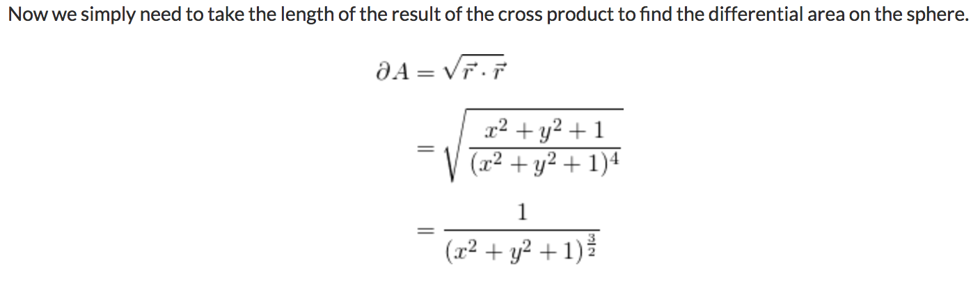
\[\frac{\partial \omega}{\partial x} \times \frac{\partial \omega}{\partial y} = \left[\begin{matrix}\frac{x}{\left(x^{2} + y^{2} + 1\right)^{2}}\\\frac{y}{\left(x^{2} + y^{2} + 1\right)^{2}}\\\frac{1}{\left(x^{2} + y^{2} + 1\right)^{2}}\end{matrix}\right]\]

…yielding the final area element

\[dA = \frac{1}{\left(x^{2} + y^{2} + 1\right)^{\frac{3}{2}}} \, dx \, dy\]

Note that this agrees with established formulas for obtaining the projected area on the sphere of a cubemap texel, as documented by, e.g. Driscoll [2012]:

Driscoll 2012 equations

Let’s do one last example before we conclude our case study. Once again, we will use cube mapping, but instead of going directly from the cube to the sphere, we will use a warp function \(f: \mathbb{R} \mapsto \mathbb{R}\) to individually pre-distort each cube face coordinate before normalizing to project onto the unit sphere. For example, we could use the warp function proposed by Everitt detailed in the previous post.

We now define \(\omega\) as

\[\omega = \frac{1}{ \sqrt{ 1 + f(x)^2 + f(y)^2 } } \, \left[ \begin{array}{c} f(x) \\ f(y) \\ 1 \end{array}\right]\]

for some arbitrary univariate function \(f\). All that’s changed since the last example is replacing \(x\) with \(f(x)\) and \(y\) with \(f(y)\). Nonetheless, if you were working by hand, at this point you might be dreading taking the partial derivatives with respect to \(x\) and \(y\) because the chain rule is going to rear its ugly head, introducing a number of extra terms to keep track of. Fortunately, SymPy will do the drudgery for us.

Here’s the minimal modification of the code. Note that we take advantage of the sympy.Function class to represent \(f\) symbolically. Why do this analysis for a particular function \(f\) when we can do it for all of them at once?

f = sympy.Function('f')
f.is_real = True

p = normalize( sympy.Matrix([f(x), f(y), 1]) )

surf3d_area_element(p, x, y)

It gives the partial derivative vectors

\[\frac{\partial \omega}{\partial x} = \left[\begin{matrix}\frac{\left(f^{2}{\left (y \right )} + 1\right) \frac{d}{d x} f{\left (x \right )}}{\left(f^{2}{\left (x \right )} + f^{2}{\left (y \right )} + 1\right)^{\frac{3}{2}}}\\- \frac{f{\left (x \right )} f{\left (y \right )} \frac{d}{d x} f{\left (x \right )}}{\left(f^{2}{\left (x \right )} + f^{2}{\left (y \right )} + 1\right)^{\frac{3}{2}}}\\- \frac{f{\left (x \right )} \frac{d}{d x} f{\left (x \right )}}{\left(f^{2}{\left (x \right )} + f^{2}{\left (y \right )} + 1\right)^{\frac{3}{2}}}\end{matrix}\right] \ ,\quad\quad\quad \frac{\partial \omega}{\partial y} = \left[\begin{matrix}- \frac{f{\left (x \right )} f{\left (y \right )} \frac{d}{d y} f{\left (y \right )}}{\left(f^{2}{\left (x \right )} + f^{2}{\left (y \right )} + 1\right)^{\frac{3}{2}}}\\\frac{\left(f^{2}{\left (x \right )} + 1\right) \frac{d}{d y} f{\left (y \right )}}{\left(f^{2}{\left (x \right )} + f^{2}{\left (y \right )} + 1\right)^{\frac{3}{2}}}\\- \frac{f{\left (y \right )} \frac{d}{d y} f{\left (y \right )}}{\left(f^{2}{\left (x \right )} + f^{2}{\left (y \right )} + 1\right)^{\frac{3}{2}}}\end{matrix}\right]\]

along with their cross product

\[\frac{\partial \omega}{\partial x} \times \frac{\partial \omega}{\partial y} = \left[\begin{matrix}\frac{f{\left (x \right )} \frac{d}{d x} f{\left (x \right )} \frac{d}{d y} f{\left (y \right )}}{\left(f^{2}{\left (x \right )} + f^{2}{\left (y \right )} + 1\right)^{2}}\\\frac{f{\left (y \right )} \frac{d}{d x} f{\left (x \right )} \frac{d}{d y} f{\left (y \right )}}{\left(f^{2}{\left (x \right )} + f^{2}{\left (y \right )} + 1\right)^{2}}\\\frac{\frac{d}{d x} f{\left (x \right )} \frac{d}{d y} f{\left (y \right )}}{\left(f^{2}{\left (x \right )} + f^{2}{\left (y \right )} + 1\right)^{2}}\end{matrix}\right]\]

and finally, the area element:

\[dA = \frac{\sqrt{\left(\frac{d}{d x} f{\left (x \right )}\right)^{2} \left(\frac{d}{d y} f{\left (y \right )}\right)^{2}}}{\left(f^{2}{\left (x \right )} + f^{2}{\left (y \right )} + 1\right)^{\frac{3}{2}}} \, dx \, dy\]

Note the derivatives \(f'(x)\) and \(f'(y)\) sitting happily up in the numerator there. If you compare this to the previous example, you can see how this one generalizes it nicely.

So there you have it, three area elements for the price of one! Hopefully by now you’ll agree that combining symbolic math with the scriptability of Python yields some interesting possibilities.

That’s all (for now)

Although I think we’ve reached a reasonable stopping point for the time being, there were a handful of issues I didn’t get to address yet in this series, including:

limits and integration
verifying equality of symbolic expressions
tips and workarounds when SymPy isn’t being helpful
comparing SymPy to other computer algebra systems

I’m not sure yet exactly which topics I’ll cover, or how many posts it’ll take to do so, so if you have particular requests or questions, please chime in on this twitter thread.

Thanks for reading!