Demystifying discrete-time linear systems

Just what is a discrete-time linear system, and what kinds of dynamical behaviors can they represent?

Overview

This is the first post in a multi-part series about controls and filtering. It’s gonna start out basic but will hopefully lead to some nuggets that could be interesting even to readers with background in estimation and controls.

With that said, if you’re already familiar with these fields you’ll likely find this particular post fairly introductory. If not, stick around and I’ll do my best to define exactly what the heck is a discrete-time linear system.

Our dumb motivating example: an ice block

Let’s start with a contrived yet classic example from the literature: a mass under externally-generated forces. Visualize a block of ice with a fan stuck to it, gliding frictionlessly across an ice rink.

No wait – I’ll visualize it for you. Let me fire up jspaint.app… ok here:

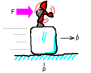
So the block of ice is at a position of \(p\) meters from some fixed reference point – say, the center line. It is currently traveling at a velocity of \(\dot{p}\) meters per second. The fan is generating a thrust force of \(F\) newtons which induces an acceleration of \(\ddot{p} = F / m\) meters per second squared, where \(m\) is the mass of the ice block.

Why is \(\ddot{p} = F/m\)? We are used to thinking about Newton’s second law of motion as \(F = ma\), but when simulating dynamical systems, we are often given the force and need to compute the acceleration, so we frequently see equations of the form \(a = F/m\).

Aside: If you’re scratching your head about the dots on top of the \(p\)’s, they denote time derivatives. Since position is \(p\) and velocity is its first derivative (i.e. \(dp/dt\)), we write velocity as \(\dot{p}\). Since acceleration is the second derivative of position, we write it as \(\ddot{p}\). You can blame Newton for all the dots – he invented this notation.

A discrete-time linear system is a way of grouping the dynamics of a particular model into a standardized matrix-vector equation. It requires you to separate variables into state (in our case, the position and velocity of the ice block) and controls (the force from the fan).

How do you know what’s in the state and what’s in the control? The rule of thumb is that if you can instantaneously change a variable yourself (i.e. generate a force by sending a particular voltage to the fan), it’s a control, and otherwise it’s a state. I can definitely use the fan to affect the position and velocity of the ice block, but only indirectly, and over time.

The other rule is that the state must include all of the variables required to model the behavior of the system. I may only care about position and not velocity, but I have to include the velocity because I can’t predict future positions without knowing something about the current velocity.

Because it’s a standardized form, every discrete-time linear system is written down as

\[\mathbf{x}_t = \mathbf{A} \mathbf{x}_{t-1} + \mathbf{B} \mathbf{u}_t\]

where \(\mathbf{x}_t \in \mathbb{R}^n\) is the current state, \(\mathbf{x}_{t-1} \in \mathbb{R}^n\) is the previous state, \(\mathbf{u}_t \in \mathbb{R}^q\) is the current control, \(\mathbf{A}: n \times n\) is the state matrix that relates the current state to the previous state, and \(\mathbf{B}: n \times q\) is the input matrix that relates the current state to the current control.

In our example, we have

\[\mathbf{x}_t = \left[\begin{array}{c} \text{position at time}\ t \\ \text{velocity at time}\ t \end{array}\right] = \left[\begin{array}{c} p_t \\ \dot{p}_t \end{array}\right]\]

and

\[\mathbf{u}_t = \left[\begin{array}{c} \text{force at time}\ t \end{array}\right] = \left[\begin{array}{c} F_t \end{array}\right] = \left[\begin{array}{c} m \, \ddot{p} \end{array}\right].\]

The plots below show what happens if we begin with an initial state of \(\mathbf{x}_0 = (0, 0.1)\) and briefly apply a force of 1 Newton (note: for simplicity’s sake all of the simulations on this page assume a mass of \(m = 1\) kg).

Note that velocity is the slope of the position graph. Velocity is initially constant at 0.1 m/s, and jumps to 0.2 m/s after the force is applied. Finally, you’ll notice that the force is zero at all times except briefly in the middle.

Play with the first slider below to change the time at which the force is applied – the graphs will update automatically.

force start time: s

force duration: s

When you’ve gotten a feel for it, set the first slider all the way left and the second slider all the way right. Now you’re looking at a mass under uniform acceleration. In this case, velocity is linearly increasing over time, and position is increasing quadratically.

But no matter how you set the sliders, the same basic relationships hold:

• velocity is the slope of the position graph, and
• force is the slope of the velocity graph.¹

To understand the underlying discrete-time linear dynamical system, we need to take these concepts about time derivatives and write them out in matrix-vector form.

Simulating dynamics = adding up lots of small changes

Given the previous position was \(p_{t-1}\) and the previous velocity was \(\dot{p}_{t-1}\), how should we compute our current position \(p_t\)? Euler’s method tells us that we can express the change in position as the rate of change (i.e. velocity) multiplied by a fixed timestep \(\Delta t\):

\[p_t = p_{t-1} + \dot{p}_{t-1} \, \Delta t.\]

Similarly, Euler’s method also tells us that the new velocity can be computed as the previous velocity plus the timestep multiplied by the rate of change in velocity – that is, the acceleration. We see that

\[\begin{align} \dot{p}_t & = \dot{p}_{t-1} + \ddot{p} \, \Delta t \\ & = \dot{p}_{t-1} + \frac{F_t}{m} \, \Delta t. \end{align}\]

Aside: Why \(F_t\) and not \(F_{t-1}\)? It’s an arbitrary decision whether controls “go with” the state they modify or the state they produce. Since the control takes place “between” the two states, it doesn’t really matter what notation we choose, as long as we are consistent. For what it’s worth, most of Wikipedia’s articles on control and estimation seem to have settled on the convention that the previous state pairs with the current control.

In order to determine the \(\mathbf{A}\) and \(\mathbf{B}\) matrices, we need to factor the previous two equations produced by Euler’s method into the matrix-vector form \(\mathbf{x}_t = \mathbf{A} \mathbf{x}_{t-1} + \mathbf{B} \mathbf{u}_t\).

After plugging in our definitions of states and controls, we find that

\[\left[\begin{array}{c} p_t \\ \dot{p}_t \end{array}\right] = \left[\begin{array}{cc} 1 & \Delta t \\ 0 & 1 \end{array}\right] \left[\begin{array}{c} p_{t-1} \\ \dot{p}_{t-1} \end{array}\right] + \left[\begin{array}{c} 0 \\ \frac{\Delta t}{m} \end{array}\right] \left[\begin{array}{c} F_t \end{array}\right].\]

I’ll rewrite the update equations for \(p_t\) and \(\dot{p}_t\) here so you can verify that they match up with the matrix equation above.

\[\begin{align} p_t & = p_{t-1} + \dot{p}_{t-1} \, \Delta t \\ \dot{p}_t & = \dot{p}_{t-1} + \frac{F_t}{m} \, \Delta t \end{align}\]

All verified? Good! We can conclude that state and input matrices for our discrete-time linear system are given by

\[\mathbf{A} = \left[\begin{array}{cc} 1 & \Delta t \\ 0 & 1 \end{array}\right] \quad\quad\text{and}\quad\quad \mathbf{B} = \left[\begin{array}{c} 0 \\ \frac{\Delta t}{m} \end{array}\right].\]

Adding in some friction

Now let’s modify our original thought experiment to consider sliding our ice block across a linoleum tile floor instead of an ice rink. Lemme fire up paint again:

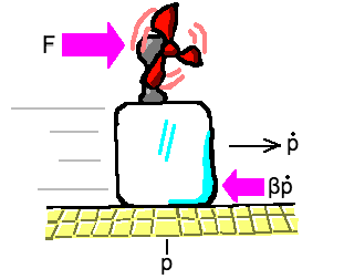
Switching from ice to linoleum, our assumption of frictionless motion is no longer valid. As the picture above shows, there are now two forces acting on the ice block: the original fan force \(F\) and a new friction force equal to \(-\beta \dot{p}\) that opposes the current velocity with a constant of proportionality \(\beta\).

Now the acceleration is given by dividing the sum of the forces acting on the block by its mass, so

\[\ddot{p} = \frac{F - \beta \dot{p}}{m}.\]

Can we reflect this in our discrete-time linear system? No problem! We’ll need to modify our velocity update equation to reflect the new definition of acceleration, paying close attention to subscripts:

\[\begin{align} \dot{p}_t & = \dot{p}_{t-1} + \ddot{p} \, \Delta t \\ & = \dot{p}_{t-1} + \frac{F_t - \beta \dot{p}_{t-1}}{m} \, \Delta t \\ & = \left(1 - \beta \tfrac{\Delta t}{m}\right) \dot{p}_{t-1} + \tfrac{\Delta t}{m} F_t. \end{align}\]

This leads us to modify the lower-right entry of the \(\mathbf{A}\) matrix (note that \(\mathbf{B}\) remains unchanged) to obtain

\[\mathbf{A} = \left[\begin{array}{cc} 1 & \Delta t \\ 0 & 1 - \beta \frac{\Delta t}{m} \end{array}\right] \quad\quad\text{and}\quad\quad \mathbf{B} = \left[\begin{array}{c} 0 \\ \frac{\Delta t}{m} \end{array}\right].\]

Let’s simulate our ice block on linoleum, setting \(\beta = 0.5\). We’ll start with initial conditions \(\mathbf{x}_0 = (0, 1)\). Also since we are focusing on just the effects of friction, we’ll leave the fan off to keep \(F = 0\) and we’ll also omit the graph of the controls.

Note that velocity is decaying exponentially towards zero as the friction bleeds off speed. In turn, you can see position exponentially converging towards a final resting position.

Here’s a slider so you can play with the friction constant:

β =

With zero friction, the ice block continues at a constant velocity forever, and as friction increases, the velocity decays faster and faster.

Making things springy

OK, to add to our increasingly contrived scenario, let’s imagine we’re back on ice but this time there’s a spring tugging the ice block back to the center line the further away the block moves from \(p = 0\).

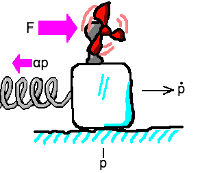
Once again, there are two forces acting on the block of ice, the fan force \(F\), and a spring force \(-\alpha p\) that acts with opposite sign to the current position, where \(\alpha\) is a spring constant.

Just like the friction example above, we can accommodate this into our discrete-time linear system by modifying our update rule for velocity, and therefore our \(\mathbf{A}\) matrix.

The new velocity update rule in this case is

\[\begin{align} \dot{p}_t & = \dot{p}_{t-1} + \ddot{p} \, \Delta t \\ & = \dot{p}_{t-1} + \frac{F_t - \alpha p_{t-1}}{m} \, \Delta t \\ & = -\alpha \tfrac{\Delta t}{m} p_{t-1} + \dot{p}_{t-1} + \tfrac{\Delta t}{m} F_t. \end{align}\]

This causes a change to the lower left entry of the state matrix, compared to the original example (again, \(\mathbf{B}\) remains unchanged):

\[\mathbf{A} = \left[\begin{array}{cc} 1 & \Delta t \\ -\alpha \frac{\Delta t}{m} & 1 \end{array}\right] \quad\quad\text{and}\quad\quad \mathbf{B} = \left[\begin{array}{c} 0 \\ \frac{\Delta t}{m} \end{array}\right].\]

Here’s a simulation with \(\alpha = 1.0\). This time we will set our initial conditions to \(\mathbf{x}_0 = (1, 0)\) – i.e. initially positioned 1 meter from the center line, with zero velocity. Like the second simulation, we’ll leave the fan turned off in this one too.

This example is also interactive, so you can use the slider below to play with the spring constant.²

α =

You’ll notice that when we add in the spring force, the motion of the ice block becomes sinusoidal, with the frequency of the back-and-forth motion of the block proportional to the spring constant. Low spring constant makes for slow waves, and high spring constant makes for fast waves. And once again we can confirm that the velocity graph shows the slope of the position graph. When position is at a maximum (or minimum), velocity is zero, and vice versa.

Putting it all together

Here’s one simulation to let you play with all three aspects together – the force from the fan, friction, and spring constant.

force start time: s

force duration: s

β = (friction)

α = (spring constant)

Note that now that we are also considering forces due to friction and the spring, the commanded force from the fan no longer exactly corresponds to the slope of the velocity plot.

What’s the point?

We’ve seen that even this simple system with two state variables and one control variable is expressive enough to represent a variety of real-world phenomena, including inertia, friction, and spring forces.

All the same, you might find it a bit cumbersome to write down the dynamics of the model in matrix-vector form when the individual update rules for position and velocity are easier to understand individually. So, why go through the trouble to do this?

For starters, separating the dynamics into a state matrix \(\mathbf{A}\) and an input matrix \(\mathbf{B}\) can help you understand what aspects are under active control (those parts live in \(\mathbf{B}\)), and what are the passive dynamics of the system that unfold whether you are actively controlling it or not (that’s \(\mathbf{A}\)). You can always turn off the active dynamics by specifying a control of zero, but your system is forever doomed to the tyranny of its own passive dynamics.

Furthermore, many well-established and thoroughly-studied tools and techniques expect you to specify a system in a standard matrix form. These include controllability analysis, which can tell you whether you can drive your system to any arbitrary state, as well as control schemes like the linear quadratic regulator (LQR) or estimation methods like the Kalman filter. I’ll be writing about all of these in future posts.

By the way, there are other standard forms to represent dynamical systems – for example the continuous-time linear system – but in my opinion you can’t beat discrete-time linear systems as an entry point into the world of estimation and control.

These types of dynamical systems are ubiquitous across all subfields of Engineering (except for perhaps Civil Engineering, where if things have appreciable velocity or acceleration you are having a Very Bad Day). We just looked at the mechanics of a sliding block of ice, but I could have just as easily brought in an electric circuit, a thermal system, or a system of chemical reactions. Being able to understand systems in a canonical or standard form means that engineers from disparate subfields can communicate with each other without having to learn too much specialized language.

Also, I just really like linear algebra so if there’s a matrix way of writing something down it’s a safe bet that it’s gonna be my go-to for thinking about the problem.

Further extensions and future posts

In a future post we’ll investigate whether we can modify our discrete-time linear system to convert horizontal propulsion to vertical propulsion that counters the constant force of gravity.

Behold, the ice-copter:

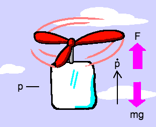
Will it fly? Can we modify our \(\mathbf{A}\) and \(\mathbf{B}\) matrices to successfully model this system? Spoilers for future post: nope – at least not without using a trick or two.

But before we get there, we’ll spend a little quality time talking about optimal control and LQR.

Stay tuned!

Postscript: tools used on this page

All of the plots above are generated using dygraphs. Linear algebra functionality is provided by enkimute’s svelte linalg.js library. There’s some minimal use of jQuery to provide interactivity and hook everything together.

1. …only because our mass is equal to 1. If it were otherwise, force would be proportional to the slope of velocity, again because \(F = ma\). But this relationship won’t always hold once we start considering more complex systems in the other sections of this post. ↩

2. Trivia: because this simulation is much https://en.wikipedia.org/wiki/Stiff_equation than the previous ones, I had to decrease \(\Delta t\) from 0.1 to 0.001 to prevent the simulation from losing accuracy. But browsers are fast, so NBD. ↩