Flow Free redux: eating SAT-flavored crow
Turns out, sometimes a hammer is not the best tool for the job.
Overview
So in my last post, I haughtily dismissed SAT as burdensome and opaque formulation for solving puzzles like Flow Free. Since then I’ve learned a few things thanks to @asmeurer, whose thought-provoking comments pointed me towards some interesting sources on the topic.
To succinctly summarize the previous post, I wrote an automated solver for the popular Flow Free mobile puzzle app in C, based on tree search. Although you can naturally frame Flow Free as a constraint satisfaction problem (CSP), I wrote that I preferred tree search instead, because:
- I spent years in grad school coding up search-based planners with A*.
- When you have a hammer, the whole world looks like a nail.
The program I presented ended up running pretty quickly, solving all of the puzzles in my test suite in under 1.6 seconds per puzzle, while weighing in in at 1,910 physical lines of C code.1
And that would have been the happy ending to the story, had asmeurer’s comments not prodded me to try out the CSP/SAT solution. The new program, written in Python, has a worst-case solution time of about 0.4 seconds on my test cases, using 3x less code than the C solver.2
Background
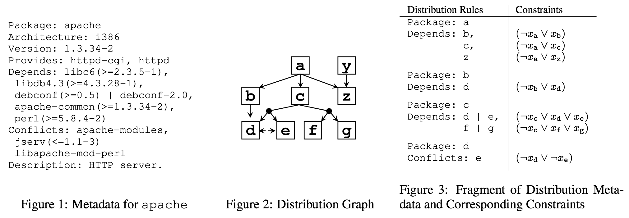
As I recently learned, dependency resolution is another problem that can also be posed as either graph search or as SAT.3 In a nutshell, the objective is to decide what additional packages to install or uninstall when a user wants to run some desired piece of software. The figures below, from this paper, show how dependency/conflict relationships between packages can be represented in both ways:
Indeed in 2013, the Python distribution Anaconda switched its conda package management tool to resolving dependencies using SAT, thanks to developer Ilan Schnell. The underlying engine is the C-based PicoSAT solver, made accessible from Python by Schnell’s pycosat module. As a warm-up to solving the dependency problem, he used pycosat to write a Sudoku solver, which was a helpful and instructive example as I began writing my pycosat-based Flow Free solver.
Conjunctive normal form
The thorniest part of reducing a general CSP to a SAT problem is that the constraints must typically be expressed in conjunctive normal form (CNF). CNF consists of a number of OR-clauses, all of which must be satisfied conjunctively (i.e. they are all AND-ed together). Each OR-clause is a disjunction over one or more literals consisting of single logical variables or their negations.
Converting to CNF can be a bit tricky: the logical statement \(x \leftrightarrow y\) (i.e. “\(x\) and \(y\) are either both true or both false”) gets represented as the two clauses
\[\begin{align} (x \lor \lnot y) \land (\lnot x \lor y) \end{align}\]whereas the Boolean exclusive-or (XOR) of the two variables, \(x \not \leftrightarrow y\), must be represented as
\[\begin{align} (x \lor y) \land (\lnot x \lor \lnot y) \end{align}\]Logical implications like \(x \rightarrow y\) become the single clause \((\lnot x \lor y)\), and negations of AND-clauses such as \(\lnot (x \land y )\) (that is, “it is not the case that both \(x\) and \(y\) are true”) are straightforwardly converted through DeMorgan’s law to \((\lnot x \lor \lnot y)\).
Reducing Flow Free to SAT
With this basic understanding of CNF, we’re ready to begin reducing Flow Free to SAT. By the way, the discussion in this section pretty much follows the recipe for a SAT-based solver outlined in the StackOverflow answer I linked to in my last post, but it fills in a lot more details that I had to figure out on on my own.
One by one, we will see how to encode the following list of constraints into CNF:
- Every cell is assigned a single color.
- The color of every endpoint cell is known and specified.
- Every endpoint cell has exactly one neighbor which matches its color.
- The flow through every non-endpoint cell matches exactly one of the six direction types.
- The neighbors of a cell specified by its direction type must match its color.
- The neighbors of a cell not specified by its direction type must not match its color.
Let’s define some variables and indices to get started. Say that our puzzle has \(N\) cells and \(C\) colors. We will use \(i\), \(j\), \(k\), \(\ldots\) to refer to to individual cells, so for instance we have cell \(i \in \{1, \ldots, N\}\). Similarly, we will use the indices \(u, v \in \{1, \ldots, C\}\) to refer to individual colors. Finally, we can define six “direction types” that specify which of a non-endpoint cell’s neighbors are connected to it by some flow (we can conveniently illustrate them with Unicode box drawing characters). The six types are:
| Direction type | Unicode char | Description |
|---|---|---|
| 1 | ─ |
left-right |
| 2 | │ |
top-bottom |
| 3 | ┘ |
top-left |
| 4 | └ |
top-right |
| 5 | ┐ |
bottom-left |
| 6 | ┌ |
bottom-right |
We will use \(t \in \{ 1, \ldots 6 \}\) to index these direction types. With that setup in mind, let’s address the first constraint on our list above.
Every cell is assigned a single color. We will create \(N \times C\) Boolean variables to encode the color of each cell: if the SAT solution sets \(x_{i,u}\) to true, that means that cell \(i\) has color \(u\). These color variables are handled slightly differently in endpoint cells (i.e. the colored dots that are initially filled in before the puzzle is solved) and normal free cells. Let’s consider normal cells first.
Clearly every cell must have some color, so for each non-endpoint cell \(i\), we can write the clause:
\[\begin{align} (x_{i,1} \lor x_{i,2} \lor \ldots \lor x_{i,C}) \end{align}\]Also, for each non-endpoint cell \(i\), we know that no two color variables can be true, so we get the clauses:
\[\begin{align} ( \lnot x_{i,1} \lor \lnot x_{i,2} ) \land ( \lnot x_{i,1} \lor \lnot x_{i,3} ) \land ( \lnot x_{i,1} \lor \lnot x_{i,4} ) \land \ldots \land ( \lnot x_{i,1} \lor \lnot x_{i,C} ) & \\ ( \lnot x_{i,2} \lor \lnot x_{i,3} ) \land ( \lnot x_{i,2} \lor \lnot x_{i,4} ) \land \ldots \land ( \lnot x_{i,2} \lor \lnot x_{i,C} ) & \\ ( \lnot x_{i,3} \lor \lnot x_{i,4} ) \land \ldots \land ( \lnot x_{i,3} \lor \lnot x_{i,C} ) & \\ \phantom{( \lnot x_{C-1,2}} \vdots \phantom{\lnot x_{p-1,C} )} & \\ ( \lnot x_{C-1,2} \lor \lnot x_{C-1,C} ) & \\ \end{align}\]Each one of these comes from negating the AND clause \(x_{i,u} \land x_{i,v}\) for two different colors \(u\) and \(v\). Note we have \(C(C-1)/2\) possible combinations of two colors for each cell.
The color of every endpoint cell is known and specified. Since their colors are specified initially, for each endpoint cell \(i\), we know its true color \(u\), so we can simply assert the clause \((x_{i,u})\). We can also specify that none of the other colors are present, so \(( \lnot x_{i,v} )\) for all \(v \ne u\).
Every endpoint cell has exactly one neighbor which matches its color. This is the neighbor through which a flow originates or terminates. Let us assume endpoint cell \(i\) has known color \(u\) and neighbor cells \(j\), \(k\), \(l\), and \(m\). Since at least one neighbor of the cell has color \(u\), we can write the clause
\[\begin{align} ( x_{j,u} \lor x_{k,u} \lor x_{l,u} \lor x_{m,u} ) \end{align}\]Furthermore, no two neighbors of the endpoint cell \(i\) both share its color, so we have \((\lnot x_{j,u} \lor \lnot x_{k,u})\), and all the other two-way combinations of the neighbors (i.e. \(j\) and \(l\), \(j\) and \(m\), \(k\) and \(l\), and so on).
The flow through every non-endpoint cell matches exactly one of the
six direction types. Now, for each non-endpoint cell we introduce up
to six Boolean “direction type” variables that specify which two
neighbors of the cell are connected to it along a solution path. If
variable \(y_{i,t}\) is true in the SAT solution, then some flow
connects cell \(i\) to the two of its neighbors specified by type
\(t\) from the table above. Note that some cells can not assume all of
the direction types – for instance, it is impossible for a flow to
have the ┘ direction type anywhere in the top row or leftmost column
of the puzzle (since those cells are missing the required neighbors
above or to the left).
Just like the color variables, we can generate clauses for the direction variables to ensure that:
- every non-endpoint cell cell has at least one direction type, and
- no two directions types are specified for any non-endpoint cell.
The former gives us one clause per cell; the latter gives up to 15 additional clauses – one for each possible pair of direction types present.
The neighbors of a cell specified by its direction type must match
its color. It’s time to consider the interaction between direction
type variables and color variables. Each direction type picks out two
neighbors of a cell; for example, direction type ┐ selects a
cell’s left neighbor and its bottom neighbor. So for any cell \(i\)
and any direction type \(t\) applied to it, we get two
neighbors \(j\) and \(k\) that must have the same color as cell
\(i\). That means, for all colors \(u\):
…bearing in mind that the indices \(j\) and \(k\) are jointly determined by the cell \(i\) and the direction type \(t\). Massaging the statement above into CNF gives us four clauses:
\[\begin{align} (\lnot y_{i,t} \lor \lnot x_{i, u} \lor x_{j, u}) \\ (\lnot y_{i,t} \lor x_{i, u} \lor \lnot x_{j, u}) \\ (\lnot y_{i,t} \lor \lnot x_{i, u} \lor x_{k, u}) \\ (\lnot y_{i,t} \lor x_{i, u} \lor \lnot x_{k, u}) \\ \end{align}\]The neighbors of a cell not specified by its direction type must not match its color. This is the constraint that prevents path self-contact. For any neighbor \(l\) of \(i\) which isn’t picked out by direction type \(t\), we can say \(y_{i,t} \rightarrow \lnot (x_{i,u} \land x_{l,u})\). In CNF, this becomes the clause
\[\begin{align} (\lnot y_{i,t} \lor \lnot x_{i, u} \lor \lnot x_{l, u}) \\ \end{align}\]…That’s it! We just generated quite a few variables and clauses: our puzzle of size \(N\) with \(C\) colors has \(NC\) color variables and about \(6 N\) direction type variables, with \(O(NC^2)\) clauses over just the color variables and an additional \(O(NC)\) clauses for direction-color interactions. You may recall that SAT runtimes are, in the worst case, exponential in the number of variables. Should we be worried about prohibitively slow solution speeds? Spoiler alert: nope.
Dealing with cycles
One point that got raised in the StackOverflow answer is that this particular reduction to SAT does not prevent freestanding cycles from arising in the puzzle. Here’s an example – on the left below, we have the initial state of a 14x14 puzzle, and on the right, an invalid solution with a cycle (the 2x2 yellow square in the top left):

Let’s double-check whether this obviously bogus solution meets our constraints from before:
- Every cell is assigned a single color. ✓
- The color of every endpoint cell is known and specified. ✓
- Every endpoint cell has exactly one neighbor which matches its color. ✓
- The flow through every non-endpoint cell matches exactly one of the six direction types. ✓
- The neighbors of a cell specified by its direction type must match its color. ✓
- The neighbors of a cell not specified by its direction type must not match its color. ✓
Unfortunately, the cycle really is allowed. Like the StackOverflow commenter, the only way I can think to prevent them in the SAT specification would be to add O(N^2) additional variables to track whether each cell is rooted the starting point of some flow. I tried going down this path, and it really bogged down the PicoSAT solver.
Instead of adding the extra “rootedness” variables, my program works
incrementally by detecting cycles in the SAT solver’s output and
emitting additional clauses to prevent them. For instance, in response
to the bogus solution on the right above, it would add a clause saying
“either cell (4, 3) is not ┌ or (4, 4) is not ┐ or (5,4) is not
┘ or (5, 3) is not └”. In other words, it is not the case that all
four cells have the direction types causing the cycle.
In the case of this particular puzzle, having been prohibited from forming the yellow cycle above, the incremental solver happily discovers one more cycle (left below) before finding the true solution (right):

It turns out that this kind of incremental solution of SAT problems, where the solver is invoked multiple times as variables and clauses are added, is an application area of sufficient interest that it now merits its own category at the yearly SAT competition.4
Conclusions
As the table below shows, although the C solver is faster than the
SAT-based Python solver on most puzzles (especially small ones), the
worst-case solution time for the Python solver is much better. Looking
at the time differences between them, the maximum in favor of the C
solver is 0.356 seconds, on jumbo_14x14_01.txt – the only puzzle in
the test suite that actually necessitates cycle detection and
repair. On the other hand, the maximum difference in favor of the
Python solver is 1.197 seconds on the slowest puzzle for the C solver,
jumbo_14x14_30.txt.
Add to that the fact that the Python program has far less code than the C version, and SAT starts to look really appealing. I’m going to close off this post with another screen grab of a Facebook exchange that I think really captures the learning experience of this week’s exercise:
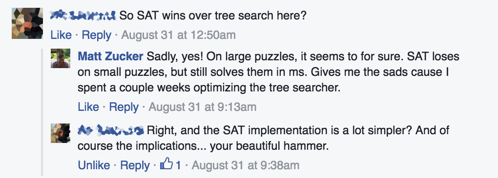
Don’t get too attached to your hammers, kids!
Appendix: experimental data
| Puzzle | # SAT vars | # clauses | Python time | C time | Difference |
|---|---|---|---|---|---|
| regular_5x5_01.txt | 184 | 2,031 | 0.003 | 0.001 | 0.002 |
| regular_6x6_01.txt | 322 | 4,353 | 0.004 | 0.001 | 0.003 |
| regular_7x7_01.txt | 452 | 6,418 | 0.007 | 0.001 | 0.006 |
| regular_8x8_01.txt | 616 | 9,452 | 0.010 | 0.001 | 0.009 |
| regular_9x9_01.txt | 1,009 | 17,595 | 0.021 | 0.001 | 0.020 |
| extreme_8x8_01.txt | 571 | 8,472 | 0.011 | 0.001 | 0.010 |
| extreme_9x9_01.txt | 661 | 9,112 | 0.017 | 0.001 | 0.016 |
| extreme_9x9_30.txt | 807 | 13,048 | 0.026 | 0.001 | 0.025 |
| extreme_10x10_01.txt | 938 | 14,818 | 0.019 | 0.034 | -0.015 |
| extreme_10x10_30.txt | 1,015 | 16,871 | 0.031 | 0.008 | 0.023 |
| extreme_11x11_07.txt | 1,361 | 24,546 | 0.054 | 0.021 | 0.033 |
| extreme_11x11_15.txt | 1,482 | 28,349 | 0.036 | 0.004 | 0.032 |
| extreme_11x11_20.txt | 1,375 | 25,248 | 0.048 | 0.001 | 0.047 |
| extreme_11x11_30.txt | 1,481 | 28,261 | 0.046 | 0.003 | 0.043 |
| extreme_12x12_01.txt | 1,786 | 34,934 | 0.053 | 0.211 | -0.158 |
| extreme_12x12_02.txt | 2,059 | 43,543 | 0.055 | 0.013 | 0.042 |
| extreme_12x12_28.txt | 1,525 | 26,949 | 0.055 | 0.823 | -0.768 |
| extreme_12x12_29.txt | 1,918 | 38,934 | 0.082 | 0.107 | 0.025 |
| extreme_12x12_30.txt | 1,670 | 31,672 | 0.071 | 0.002 | 0.069 |
| jumbo_10x10_01.txt | 1,565 | 31,645 | 0.043 | 0.001 | 0.042 |
| jumbo_11x11_01.txt | 1,928 | 41,143 | 0.051 | 0.001 | 0.050 |
| jumbo_12x12_30.txt | 2,597 | 59,919 | 0.086 | 0.002 | 0.084 |
| jumbo_13x13_26.txt | 2,934 | 69,591 | 0.097 | 0.149 | -0.052 |
| jumbo_14x14_01.txt | 3,787 | 94,498 | 0.359 | 0.003 | 0.356 |
| jumbo_14x14_02.txt | 3,056 | 70,258 | 0.093 | 0.886 | -0.793 |
| jumbo_14x14_19.txt | 3,229 | 75,551 | 0.155 | 1.238 | -1.083 |
| jumbo_14x14_21.txt | 3,973 | 100,758 | 0.138 | 0.018 | 0.120 |
| jumbo_14x14_30.txt | 3,785 | 94,180 | 0.361 | 1.558 | -1.197 |
Comments
The nice thing about the SAT writeup you've done is that it should be possible to add a few constraints to handle the "Flow Free Bridges" puzzles by specifying the cells that are the bridges and changing your "The flow through every non-endpoint cell matches exactly one of the six direction types" condition into two conditions: "The flow through every non-endpoint/non-bridge cell matches exactly one of the six direction types" and "The flow through every bridge cell matches both the up/down and left/right direction types and no others."
Left as an exercise for the reader :)
But then reader has to figure out your code first. Reader has other things to do :)
Maybe another reader. I think this blog has at least two
You'd also have to relax the "Every cell is assigned a single color" constraint for bridge nodes to be "Every non-bridge cell is assigned a single color" and "Every bridge cell is assigned two colors."
Very nice!
The solver in conda also works somewhat incrementally, although I'm not sure if it counts as the same thing for the SAT competition. As I mentioned in other comment (https://mzucker.github.io/2016..., dependency resolution ends up being an optimization problem (you don't just want to install a satisfiable set of packages, you want to install the newest compatible versions possible). Conda represents the versions of packages installed as a linear integer formula, which is minimized for newer versions. This is converted to SAT via binary decision diagram (BDD) (another method which is also implemented is sorter networks, see "Translating Pseudo-Boolean Constraints into SAT," Eén and Sörensson). It then becomes a matter of bisecting the right-hand side of the equation (regenerating the formula to CNF each time and solving it with the package dependency constraints) until the minimal value is found. This part of conda was written by me in 2014-2015.
-
Code sizes computed using David A. Wheeler’s SLOCCount. ↩
-
Not exactly an apples-to-apples comparison. The C version emits SVGs (Python doesn’t), and has a lot more debugging and visualization features in general. But still. ↩
-
The implication that DLL hell is effectively considered to be an NP-hard problem is sad, but unsurprising in hindsight. ↩
-
You knew there was a yearly SAT competition, right? ↩
Comments are closed, see here for details.