Tips and tricks for being an effective (aka lazy) mathematical programmer.

If you’re looking for a basic tutorial of SymPy, this is not the best place to begin. Instead, my goal is to provide a series of case studies of actual instances where I’ve used symbolic math in “real-world” projects.¹ Part 1 (this post) will cover equation solving using SymPy. A future post will delve further into derivatives and gradients.

Update: part 2 and part 3 of this series have now been posted.

Who should read this, what’s SymPy, and why do I care?

This series of posts assumes a working knowledge of linear algebra, trigonometry, and derivatives, as well as familiarity with programming in Python. The target audience is coders working in math-heavy domains who occasionally need to:

solve systems of (possibly nonlinear) equations
figure out expressions for derivatives and gradients
verify their code agrees with an analytic solution

I routinely use SymPy to do all of these. From its own description,

SymPy is a Python library for symbolic mathematics. It aims to become a full-featured computer algebra system (CAS) while keeping the code as simple as possible in order to be comprehensible and easily extensible. SymPy is written entirely in Python.

The crux of symbolic mathematics is defining variables that, instead of storing a particular integer or string, are abstract placeholders for mathematical quantities. We can reason about these placeholder variables just as we can reason about the equation \(y = mx + b\) without needing to know the particlar values of \(y\), \(m\), \(x\) or \(b\).

Getting started with symbolic math can be awkward because it goes against our experience as programmers of a variable being a “storage slot” that holds a concrete value; however, it’s a powerful framework because abstract symbol manipulation is exactly how we do pencil-and-paper math.

You can think of a Computer Algebra System (CAS) as combining these symbols with a set of production rules or inference rules that represent the laws of mathematics. So if you feed your CAS an equation of the form \(3x = 12y\), it “knows” that it can multiply both sides by \(\frac{1}{3}\) to obtain \(x = 4y\).

Now add to that knowledge every trig identity you’ve ever forgotten from high school, all of the exp/log identities, rules for limits, derivatives (including chain rule, product rule, etc.) and integrals, and you can begin to see why this type of software might be particularly useful.

Case study 1: finding the general form of a function and its inverse

When I was studying approximately area-preserving cube-to-sphere projections for cool procedural texturing applications, I came across a function designed by Cass Everitt designed to prewarp cube faces in order to equalize projected area for cubemap textures.

I like this cube distortion function. Better sampling in the center of each face, and hardware cheap. pic.twitter.com/8Yj5lkquXV
— Cass Everitt (@casseveritt) January 1, 2015

In case you can’t see the tweet above, the forward and inverse functions are given by:

\[\begin{align} y & = 1.5x - 0.5 x^2 \\ x & = 1.5 - 0.5 \sqrt{ 9 - 8y } \end{align}\]

(Note I swap the roles of \(x\) and \(y\) in the second equation to make the forward/inverse relationship clearer.) Everitt also has a github repo where you can find a similar-looking forward/inverse pair:

\[\begin{align} y & = 1.375 x - 0.375 x^2 \\ x & = 1.833333 - 0.16666667 \sqrt{ 121.0 - 96.0 y } \end{align}\]

Looking at these two pairs, I suspected they were two particular cases of some more general formula.

Goal: derive the general formula for the forward and inverse mapping from these two examples.

Well, looking at the forward equations, we can guess that the general form for the forward function is

\[y = k x - (k - 1) x^2\]

for some \(k > 1\). Actually, that makes sense for the domain \([0, 1]\) because when \(x = 0\), we get \(y = 0\), and when \(x = 1\) we get \(y = 1\), so the center and edge of the cube map are fixed in place.

What’s the inverse of this little quadratic function? We could find it by hand, but let’s just fire up SymPy:

from __future__ import print_function # still using Python 2.7
import sympy

# create a symbolic variable for each symbol in our equation
y, x, k = sympy.symbols('y, x, k', real=True)

# define the equation y = kx - (1-k)x^2
fwd_equation = sympy.Eq(y, k*x - (k - 1)*x**2)

# solve the equation for x and print solutions
inverse = sympy.solve(fwd_equation, x)
print('found {} solutions for x:'.format(len(inverse)))
print('\n'.join([str(s) for s in inverse]))

It outputs

found 2 solutions for x:
(k - sqrt(k**2 - 4*k*y + 4*y))/(2*(k - 1))
(k + sqrt(k**2 - 4*k*y + 4*y))/(2*(k - 1))

Let’s see how that first solution looks when we substitute in \(k = 1.5\) or \(k = 1.375\):

print(inverse[0].subs(k, 1.5).simplify())
print(inverse[0].subs(k, 1.375).simplify())

This gives

-1.0*sqrt(-2.0*y + 2.25) + 1.5
-1.33333333333333*sqrt(-1.5*y + 1.890625) + 1.83333333333333

Although these aren’t identical to the formulas Everitt provides, plotting them over the \([0, 1]\) range for \(y\) reveals they are equivalent. So we’ve accomplished our goal of finding the general forward and inverse functions.

Let’s conclude this example with a nice trick for any users of LaTeX or MathJax: we’ll ask SymPy to typeset the inverse formula for us.

print('x =', sympy.latex(inverse[0]))

It gives the output

x = \frac{1}{2 \left(k - 1\right)} \left(k - \sqrt{k^{2} - 4 k y + 4 y}\right)

The result looks like this:

\[x = \frac{1}{2 \left(k - 1\right)} \left(k - \sqrt{k^{2} - 4 k y + 4 y}\right)\]

Now you can write a Python script to spit its output directly into your next graphics paper!

Case study 2: solving systems of equations

For my Wythoff explorer shader on Shadertoy (pictured below),

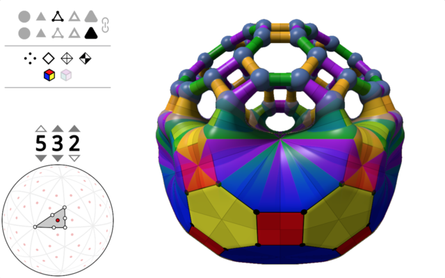
all of the rendering begins by constructing a triangle on the unit sphere with angles of \(p\), \(q\), and \(r\) (these angles are set by the spin boxes surrounding the numbers in the graphic above). Call the corresponding vertices of this triangle \(P\), \(Q\), and \(R\).

Goal: solve for these vertices such that the desired angles are formed.

The sides of a spherical triangle on the unit sphere can be represented as planes passing through the origin, therefore we can represent each side using only its unit-length normal vector \(\ell\). Call the three sides \(\ell_P\), \(\ell_Q\), and \(\ell_R\) according to which angle they lie opposite from.

To pin down the triangle on the sphere, let’s fix \(P = (0, 0, 1)\) and also fix \(\ell_R = (1, 0, 0)\) to be normal to the \(x\)-axis. Note that \(\ell_R\) passes through \(P\) by construction because \(P \bullet \ell_R = 0\). Overall, the situation looks like this:

a spherical triangle diagram

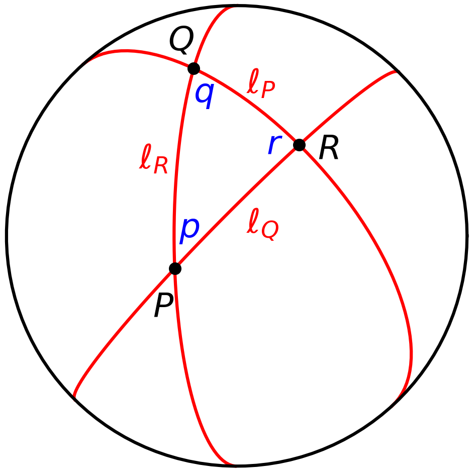
Our solution strategy will be to find the remaining sides of the triangle \(\ell_Q\) and \(\ell_P\), and then solve for the points from there because we can just write

\[Q = \frac{\ell_P \times \ell_R}{\| \ell_P \times \ell_R \|}\ , \quad\quad\quad R = \frac{\ell_Q \times \ell_P}{\| \ell_Q \times \ell_P \|}\]

That is, \(Q\) and \(R\) are the unit vectors lying on the intersections of the respective edges shown above.

So now let’s solve for \(\ell_Q = (x_1, y_1, z_1)\). We will tell SymPy to find the values of \(x_1, y_1, z_1\) that satisfy three constraints:

the edge \(\ell_Q\) contains \(P\).
the dihedral angle formed by the planes with normals \(\ell_Q\) and \(\ell_R\) is \(p\).
\(\ell_Q\) is a unit vector.

Note that taking the dot product of two planes’ normal vectors gives the negative cosine of their dihedral angle, so the middle constraint above can be expressed as \(\ell_Q \bullet \ell_R = -\cos p\). Here’s the corresponding SymPy code:

from __future__ import print_function # still using Python 2.7
import sympy

# create some symbols for angles
p, q, r = sympy.symbols('p, q, r', real=True)

# create some symbols for unknown elements of lQ
x1, y1, z1 = sympy.symbols('x1, y1, z1')

# define vectors we know so far
P = sympy.Matrix([0, 0, 1])
lR = sympy.Matrix([1, 0, 0])
lQ = sympy.Matrix([x1, y1, z1])

lQ_equations = [
    sympy.Eq(lQ.dot(P), 0),              # lQ contains P
    sympy.Eq(lQ.dot(lR), -sympy.cos(p)), # angle at point P
    sympy.Eq(lQ.dot(lQ), 1)              # lQ is a unit vector
]

S = sympy.solve(lQ_equations, x1, y1, z1, dict=True, simplify=True)
print('found {} solutions for lQ:'.format(len(S)))
print('\n'.join([sympy.pretty(sln) for sln in S])) # ask for pretty output

lQ = lQ.subs(S[1])
print('now lQ is {}'.format(lQ))

…and its output (note fancy Unicode subscripts thanks to sympy.pretty):

found 2 solutions for lQ:
{x₁: -cos(p), y₁: -│sin(p)│, z₁: 0}
{x₁: -cos(p), y₁: │sin(p)│, z₁: 0}
now lQ is Matrix([[-cos(p)], [Abs(sin(p))], [0]])

A couple notes about the code above: we define symbols using real=True because it enables some trigonometric simplifications that SymPy won’t apply if it thinks variables might be complex numbers (which is the default assumption). Also we provide sympy.solve the options dict=True and simplify=True – the former provides the solutions as a list of Python dictionaries that are easy to use with subs, and the latter because it applies useful trig identities like \(\cos^2 \theta + \sin^2 \theta = 1\) (which was actually needed to get a succinct solution here).

One of SymPy’s quirks is that it sometimes adds extraneous details to solutions like the absolute value above (not needed here because \(\pm \sin p\) and \(\pm | \sin p |\) are equivalent sets of values). Removing these is quick once you notice them. Here’s the code to get rid of the stray Abs:

lQ = lQ.subs(sympy.Abs(sympy.sin(p)), sympy.sin(p))
print('after subbing out abs, lQ is {}'.format(lQ))

…once more, the output:

after subbing out abs, lQ is Matrix([[-cos(p)], [sin(p)], [0]])

This raises the important point that using a CAS is not always a turn-key operation. It’s better to think of it more as a collaboration or conversation between you and the computer. It’s great at blindly applying rules, but doesn’t always know exactly what you want. So you write your program incrementally, working with the CAS as you go. It’s the perfect use case for the read-eval-print loop (REPL) or even an interactive Python shell like Jupyter Notebook.

Anyways, let’s manually verify that the solution worked. This is absolutely unnecessary because sympy.solve doesn’t return incorrect solutions, but it can be a nice sanity check, and the code is short, anyways:

print('checking our work:')
print('  lQ . P  =', lQ.dot(P))
print('  lQ . lR =', lQ.dot(lR))
print('  lQ . lQ =', lQ.dot(lQ)))

Gives the output:

  lQ . P  = 0
  lQ . lR = -cos(p)
  lQ . lQ = sin(p)**2 + cos(p)**2

Oops, looks like that last item could be simplified. Let’s try that again:

print('  lQ . lQ =', lQ.dot(lQ).simplify())

It yields

  lQ . lQ = 1

Phew. All the constraints were satisfied, and I got to show you sympy.simplify in action.

Now we can go through a similar process to solve for \(\ell_P\), except this time we will explicitly encode the unit-length constraint into its \(z\)-coordinate.²

x2, y2 = sympy.symbols('x2, y2')
z2 = sympy.sqrt(1 - x2**2 - y2**2)

lP = sympy.Matrix([x2, y2, z2])
print('||lP||^2 =', lP.dot(lP))

lP_equations = [
    sympy.Eq(lP.dot(lR), -sympy.cos(q)),
    sympy.Eq(lP.dot(lQ), -sympy.cos(r)),
]

S = sympy.solve(lP_equations, x2, y2, dict=True, simplify=True)
print('got {} solutions for lP'.format(len(S)))
print('\n'.join([sympy.pretty(sln) for sln in S]))

lP = lP.subs(S[0])
print('now lP is {}'.format(lP))

And the output (now with fancy ASCII fractions thanks to sympy.pretty):

||lP||^2 = 1
got 1 solutions for lP
⎧                 -(cos(p)⋅cos(q) + cos(r)) ⎫
⎨x₂: -cos(q), y₂: ──────────────────────────⎬
⎩                           sin(p)          ⎭
now lP is Matrix([[-cos(q)], [-(cos(p)*cos(q) + cos(r))/sin(p)], [sqrt(-(cos(p)*cos(q) + cos(r))**2/sin(p)**2 - cos(q)**2 + 1)]])

Here’s the relvant GLSL snippet from the shader linked above, reflecting the full solution we obtained:

vec3 lr = vec3(1, 0, 0);
vec3 lq = vec3(-cp, sp, 0);
vec3 lp = vec3(-cq, -(cr + cp*cq)/sp, 0);
lp.z = sqrt(1.0 - dot(lp.xy, lp.xy));

vec3 P = normalize(cross(lr, lq));
vec3 Q = normalize(cross(lp, lr));
vec3 R = normalize(cross(lq, lp));

Yeah, I know this is all fundamentally linear algebra and trig, but for me, coding it up in SymPy can be much faster than pencil-and-paper derivation, and it’s guaranteed to be correct – provided I set up the problem faithfully in the first place.

Next time…

That’s the end of part 1! Next time we’re going to take an in-depth look at using SymPy to compute symbolic derivatives and gradients, with applications in nonlinear least squares and deriving probability density functions. Stay tuned!

Questions/comments? Chime in on this twitter thread!

…to the extent that making pretty pictures on a computer screen is a “real-world” use-case. ↩
If we specified this constraint as a third equation and unknown, SymPy would find multiple solutions; this just gives us a single, more concise expression. ↩