SymPy case studies, part 2: derivatives
Using SymPy to help with single variable and multivariable derivatives.
If you’re just joining us, I recommend reading Part 1 of this series before this one to get some background and to read over case studies 1 & 2.
If you came here eager to read about deriving PDF’s, you’ll have to wait until tomorrow’s post because once again, I found I had more to write than would fit in a single post. So today, I’m going to cover automatically generating gradient code (complete with common subexpression elimination!), and tomorrow I’ll be going over some more advanced applications of derivatives in SymPy (see part 3).
Motivation: automatic differentiation in machine learning
I’m definitely not the first person to claim this, but I’m confident that some of the recent rapid gains in machine learning have been enabled by the fact that automatic differentiation is finally a solved problem for ML.
See, it used to be that in the bad old days before machine learning frameworks like Torch, Theano, Tensorflow, etc., if you wanted to code up some interesting novel neural network architecture or maximum likelihood estimator, you had to write down its loss function (think along the lines of error rate for classification, or sum of squared errors for regression), and begin the tedious process of working out all of its partial deriviatives with respect to each input, in order to correctly adjust network weights to decrease loss.
Although the process can be fairly mechanical, it’s notable that it took 15 years to get from Frank Rosenblatt’s circa-1960 invention of the perceptron to Paul Werbos’ subsequent invention of backpropagation in 1974 that enabled effective learning in multilayer perceptrons.1
Nowadays you just specify the loss function to one of the afforementioned ML frameworks and it does the rest for you. You can crank out a dozen harebrained network architectures a day without breaking a sweat! Automatic differentiation is a critical part of the great democratization of machine learning.2
Refresher: derivatives of univariate and multivariable functions
Note: Feel free to skip this section if you’re comfortable with parital derivatives and gradients and you know how to take derivatives in SymPy.
Before we continue on to our next case study, let’s take a second to (re-)familiarize ourselves with some basic definitions. I’m assuming readers are familiar with taking derivatives of functions like
\[f(x) = \exp\left(-\frac{x^2}{2}\right) \, \cos(\pi x)\]In this case, we can ask SymPy to take the derivative for us:
x = sympy.Symbol('x', real=True)
f = sympy.exp(-x**2 / 2) * sympy.cos(sympy.pi*x)

dfdx = f.diff(x) # <- yes, taking derivatives is this easy!

print("f'(x) =", sympy.latex(sympy.simplify(dfdx))
prints
\[f'(x) = - \left(x \cos{\left (\pi x \right )} + \pi \sin{\left (\pi x \right )}\right) e^{- \frac{x^{2}}{2}}\]For functions of more than one variable, we can take partial derivatives for one variable at a time by treating the remaining variables as constants. Let’s define the function
\[g(x,y) = \exp \left( -\frac{x^2 + y^2}{2} \right) \, \cos(\pi x)\]and get its partial derivatives with respect to \(x\) and \(y\). SymPy doesn’t much care whether you are taking the derivative of a single-variable expression or a multi-variable expression – all you have to do is tell it the variable of interest for differentiating:
x, y = sympy.symbols('x, y', real=True)
g = sympy.exp(-(x**2 + y**2) / 2) * sympy.cos(sympy.pi*x)

for var in [x, y]:
    print("\\frac{\\partial g}{\\partial " + str(var) + "} =",
          sympy.latex(sympy.simplify(g.diff(var))))
outputs
\[\begin{align} \frac{\partial g}{\partial x} & = - \left(x \cos{\left (\pi x \right )} + \pi \sin{\left (\pi x \right )}\right) e^{- \frac{x^{2}}{2} - \frac{y^{2}}{2}} \\[1em] \frac{\partial g}{\partial y} & = - y e^{- \frac{x^{2}}{2} - \frac{y^{2}}{2}} \cos{\left (\pi x \right )} \end{align}\]For an arbitrary function \(f(x_1, x_2, \ldots, x_n): \mathbb{R}^n \mapsto \mathbb{R}\), we define the gradient of \(f\) as the mapping \(\nabla f: \mathbb{R}^n \mapsto \mathbb{R}^n\) of partial derivatives:
\[\nabla f(x_1, x_2, \ldots, x_n) = \left[ \begin{array}{c} \frac{\partial f}{\partial x_1} \\ \frac{\partial f}{\partial x_2} \\ \vdots \\ \frac{\partial f}{\partial x_n} \\ \end{array}\right]\]Just like the derivative of a univariate function \(f(x)\) is itself a function \(f'(x)\) that can be evaluated at a particular \(x\), the gradient of a multivariable function \(f(x_1, \ldots x_n)\) is a vector-valued function \(\nabla f(x_1, \ldots, x_n)\) that can be evaluted for a particular vector of inputs \(x_1, \ldots, x_n\).
If you’ve never thought about derivatives of multivariable functions before, gradients and partial derivatives can seem intimidating, but SymPy is here to help! One of the best parts of using SymPy is never having to take a single derivative yourself.
Case study 3: Jacobians for nonlinear least squares
Today, we’re going to look at gradient computation for the image fitting C++ program that I previously documented on this site. The program aimed to approximate arbitrary grayscale images as a summation of Gabor functions parameterized by \(\theta = \left( u, v, h, s, t, \ell, \phi, \rho \right) \in \mathbb{R}^8\), defined as
\[\begin{align} f(\theta, x, y) &= h \exp \left( -\frac{x'^2}{2 s^2} -\frac{y'^2}{2 t^2} \right) \cos \left( \frac{ 2 \pi }{ \ell} x' + \phi \right) \ , & &\text{where} \\ x' &= \phantom{-}(x - u) \cos \rho + (y - v) \sin \rho & &\text{and} \\ y' &= -(x - u) \sin \rho + (y - v) \cos \rho \end{align}\]Assuming that the input image \(I\) contains \(n\) pixels, the intensity of the reconstructed image \(\tilde{I}\) at pixel location \(i \in \{ 1, \ldots, n \}\) is given by a summation of \(T\) Gabor functions:
\[\tilde{I}(x_i, y_i) = \sum_{t=1}^T f (\theta_t, x_i, y_i)\]Here’s example output for an input image of Zsa Zsa Gabor:
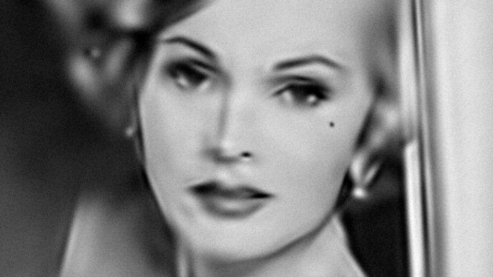
We produced this by greedily solving a sequence of nonlinear least squares problems using the levmar library written by Manolis Lourakis. In our problem, we choose \(\theta_t\) to minimize the squared norm
\[\ell_t = \| \mathbf{e}_{t-1} - \mathbf{f}(\theta_{t}) \|^2\]Here, \(\mathbf{e}_{t-1} \in \mathbb{R}^n\) is the difference between the input image and the approximation constructed so far at iteration \(t - 1\), whose \(i^{\text{th}}\) element is given by
\[e_i = I(x_i, y_i) - \sum_{j=1}^{t-1} f(\theta_j, x_i, y_i)\]The remaining term \(\mathbf{f}: \mathbb{R}^8 \mapsto \mathbb{R}^n\) is the Gabor function evaluated at each pixel location, whose \(i^{\text{th}}\) element is given by
\[f_i = f(\theta_t, x_i, y_i)\]We supply the levmar library with the vector \(\mathbf{e}_{t-1}\) and the function \(\mathbf{f}\), and let it do the hard work of finding the optimal vector of parameters \(\theta_t\). However, levmar works best when we also supply it with the \(n \times 8\) Jacobian matrix whose rows are the gradients of the \(f_i\)’s above with respect to \(\theta_t\):
\[\mathbf{J}_{\mathbf{f}}(\theta_t) = \left[ \begin{array}{c} \nabla f_1( \theta_t )^T \\ \nabla f_2( \theta_t )^T \\ \vdots \\ \nabla f_m( \theta_t )^T \end{array}\right]\]And remember, as effective (lazy) mathematical programmers, the last thing we want to do is to derive the gradient by hand.
Goal: get SymPy to automatically compute the gradient of the Gabor function with respect to \(\theta\).
This is exactly the problem that we introduced the blog post with – working out the partial derivatives of a complicated loss function – and indeed if I were re-implementing this program in 2018, I would just use TensorFlow and be done with it.3 Instead, I actually did derive the gradient terms using SymPy.
We start by just implementing the function \(f(\theta, x, y)\) defined above:
from __future__ import print_function
import sympy

x, y, u, v, h, s, t, l, rho, phi = sympy.symbols(
    'x, y, u, v, h, s, t, l, rho, phi', real=True)

cr = sympy.cos(rho)
sr = sympy.sin(rho)

xp =  (x - u) * cr + (y - v) * sr
yp = -(x - u) * sr + (y - v) * cr

f = ( h * sympy.exp(-xp**2 / (2*s**2) - yp**2 / (2*t**2) ) *
      sympy.cos( 2 * sympy.pi * xp / l + phi ) )
Next, we can just print out the partial derivatives, one by one. Since we are targeting a C++ program, we can ask SymPy to directly emit C code:
theta = (u, v, h, s, t, l, rho, phi)

for i, var in enumerate(theta):
    deriv = f.diff(var)
    print('grad[{}]'.format(i), '=', sympy.ccode(deriv) + ';')
Here’s the awful, horrible, disgusting output:
// autogenerated code, scroll right forever ----------->
grad[0] = h*(-((u - x)*sin(rho) + (-v + y)*cos(rho))*sin(rho)/pow(t, 2) + ((-u + x)*cos(rho) + (-v + y)*sin(rho))*cos(rho)/pow(s, 2))*exp(-1.0L/2.0L*pow((u - x)*sin(rho) + (-v + y)*cos(rho), 2)/pow(t, 2) - 1.0L/2.0L*pow((-u + x)*cos(rho) + (-v + y)*sin(rho), 2)/pow(s, 2))*cos(phi + 2*M_PI*((-u + x)*cos(rho) + (-v + y)*sin(rho))/l) + 2*M_PI*h*exp(-1.0L/2.0L*pow((u - x)*sin(rho) + (-v + y)*cos(rho), 2)/pow(t, 2) - 1.0L/2.0L*pow((-u + x)*cos(rho) + (-v + y)*sin(rho), 2)/pow(s, 2))*sin(phi + 2*M_PI*((-u + x)*cos(rho) + (-v + y)*sin(rho))/l)*cos(rho)/l;
grad[1] = h*(((u - x)*sin(rho) + (-v + y)*cos(rho))*cos(rho)/pow(t, 2) + ((-u + x)*cos(rho) + (-v + y)*sin(rho))*sin(rho)/pow(s, 2))*exp(-1.0L/2.0L*pow((u - x)*sin(rho) + (-v + y)*cos(rho), 2)/pow(t, 2) - 1.0L/2.0L*pow((-u + x)*cos(rho) + (-v + y)*sin(rho), 2)/pow(s, 2))*cos(phi + 2*M_PI*((-u + x)*cos(rho) + (-v + y)*sin(rho))/l) + 2*M_PI*h*exp(-1.0L/2.0L*pow((u - x)*sin(rho) + (-v + y)*cos(rho), 2)/pow(t, 2) - 1.0L/2.0L*pow((-u + x)*cos(rho) + (-v + y)*sin(rho), 2)/pow(s, 2))*sin(rho)*sin(phi + 2*M_PI*((-u + x)*cos(rho) + (-v + y)*sin(rho))/l)/l;
grad[2] = exp(-1.0L/2.0L*pow((u - x)*sin(rho) + (-v + y)*cos(rho), 2)/pow(t, 2) - 1.0L/2.0L*pow((-u + x)*cos(rho) + (-v + y)*sin(rho), 2)/pow(s, 2))*cos(phi + 2*M_PI*((-u + x)*cos(rho) + (-v + y)*sin(rho))/l);
grad[3] = h*pow((-u + x)*cos(rho) + (-v + y)*sin(rho), 2)*exp(-1.0L/2.0L*pow((u - x)*sin(rho) + (-v + y)*cos(rho), 2)/pow(t, 2) - 1.0L/2.0L*pow((-u + x)*cos(rho) + (-v + y)*sin(rho), 2)/pow(s, 2))*cos(phi + 2*M_PI*((-u + x)*cos(rho) + (-v + y)*sin(rho))/l)/pow(s, 3);
grad[4] = h*pow((u - x)*sin(rho) + (-v + y)*cos(rho), 2)*exp(-1.0L/2.0L*pow((u - x)*sin(rho) + (-v + y)*cos(rho), 2)/pow(t, 2) - 1.0L/2.0L*pow((-u + x)*cos(rho) + (-v + y)*sin(rho), 2)/pow(s, 2))*cos(phi + 2*M_PI*((-u + x)*cos(rho) + (-v + y)*sin(rho))/l)/pow(t, 3);
grad[5] = 2*M_PI*h*((-u + x)*cos(rho) + (-v + y)*sin(rho))*exp(-1.0L/2.0L*pow((u - x)*sin(rho) + (-v + y)*cos(rho), 2)/pow(t, 2) - 1.0L/2.0L*pow((-u + x)*cos(rho) + (-v + y)*sin(rho), 2)/pow(s, 2))*sin(phi + 2*M_PI*((-u + x)*cos(rho) + (-v + y)*sin(rho))/l)/pow(l, 2);
grad[6] = h*(-1.0L/2.0L*((u - x)*sin(rho) + (-v + y)*cos(rho))*(2*(u - x)*cos(rho) - 2*(-v + y)*sin(rho))/pow(t, 2) - 1.0L/2.0L*(-2*(-u + x)*sin(rho) + 2*(-v + y)*cos(rho))*((-u + x)*cos(rho) + (-v + y)*sin(rho))/pow(s, 2))*exp(-1.0L/2.0L*pow((u - x)*sin(rho) + (-v + y)*cos(rho), 2)/pow(t, 2) - 1.0L/2.0L*pow((-u + x)*cos(rho) + (-v + y)*sin(rho), 2)/pow(s, 2))*cos(phi + 2*M_PI*((-u + x)*cos(rho) + (-v + y)*sin(rho))/l) - 2*M_PI*h*(-(-u + x)*sin(rho) + (-v + y)*cos(rho))*exp(-1.0L/2.0L*pow((u - x)*sin(rho) + (-v + y)*cos(rho), 2)/pow(t, 2) - 1.0L/2.0L*pow((-u + x)*cos(rho) + (-v + y)*sin(rho), 2)/pow(s, 2))*sin(phi + 2*M_PI*((-u + x)*cos(rho) + (-v + y)*sin(rho))/l)/l;
grad[7] = -h*exp(-1.0L/2.0L*pow((u - x)*sin(rho) + (-v + y)*cos(rho), 2)/pow(t, 2) - 1.0L/2.0L*pow((-u + x)*cos(rho) + (-v + y)*sin(rho), 2)/pow(s, 2))*sin(phi + 2*M_PI*((-u + x)*cos(rho) + (-v + y)*sin(rho))/l);
Is it correct? Definitely! Would I ever use this in an actual program? Never!
The major problem here is that the code above contains excessive amounts of repeated computation, owing to both the chain rule/product rule and to the fact that transcendental functions like \(\sin\), \(\cos\), and \(\exp\) tend to appear in their own derivatives. A good C++ compiler can mitigate this through common subexpression elimination, but there’s no need to subject the compiler to that type of abuse.
Instead, we will get SymPy to do the common subexpression elimination
for us using sympy.cse:
derivs = [ f.diff(var) for var in theta ]

variable_namer = sympy.numbered_symbols('sigma_')
replacements, reduced = sympy.cse(derivs, symbols=variable_namer)

for key, val in replacements:
    print('double', key, '=', sympy.ccode(val) + ';')

print()

for i, r in enumerate(reduced):
    print('grad[{}]'.format(i), '=', sympy.ccode(r) + ';')
Here is the resulting C code:
double sigma_0 = cos(rho);
double sigma_1 = 1.0/l;
double sigma_2 = -u + x;
double sigma_3 = sin(rho);
double sigma_4 = -v + y;
double sigma_5 = sigma_0*sigma_2 + sigma_3*sigma_4;
double sigma_6 = phi + 2*M_PI*sigma_1*sigma_5;
double sigma_7 = sin(sigma_6);
double sigma_8 = pow(s, -2);
double sigma_9 = pow(sigma_5, 2);
double sigma_10 = pow(t, -2);
double sigma_11 = u - x;
double sigma_12 = sigma_0*sigma_4;
double sigma_13 = sigma_11*sigma_3 + sigma_12;
double sigma_14 = pow(sigma_13, 2);
double sigma_15 = exp(-1.0L/2.0L*sigma_10*sigma_14 - 1.0L/2.0L*sigma_8*sigma_9);
double sigma_16 = M_PI*h*sigma_15*sigma_7;
double sigma_17 = sigma_5*sigma_8;
double sigma_18 = sigma_10*sigma_13;
double sigma_19 = cos(sigma_6);
double sigma_20 = h*sigma_15*sigma_19;
double sigma_21 = 2*M_PI*h*sigma_1*sigma_15*sigma_7;
double sigma_22 = sigma_12 - sigma_2*sigma_3;

grad[0] = 2*sigma_0*sigma_1*sigma_16 + sigma_20*(sigma_0*sigma_17 - sigma_18*sigma_3);
grad[1] = sigma_20*(sigma_0*sigma_18 + sigma_17*sigma_3) + sigma_21*sigma_3;
grad[2] = sigma_15*sigma_19;
grad[3] = sigma_20*sigma_9/pow(s, 3);
grad[4] = sigma_14*sigma_20/pow(t, 3);
grad[5] = 2*sigma_16*sigma_5/pow(l, 2);
grad[6] = sigma_20*(-sigma_17*sigma_22 - sigma_18*(sigma_0*sigma_11 - sigma_3*sigma_4)) - sigma_21*sigma_22;
grad[7] = -h*sigma_15*sigma_7;
Although I would quibble with a few aspects of the code above
(unimaginative variable names, gratuitous use of pow to square or
cube numbers, using long doubles 1.0L/2.0L where a simple 0.5
would do4), it’s nonetheless far superior to the previous attempt.
A small amount of cleanup work will turn this into a program I
wouldn’t be ashamed to have on my github.
So to conclude: not only will SymPy work out your gradients for you, it will directly implement them in semi-reasonable-looking C code! It would be worth it at twice the price.5
By the way, automatic differentiation (AD) is topic of sufficient complexity to merit its own graduate-level course. There are a number of alternatives to SymPy for AD. One promising-looking one that I have yet to try is autograd, which operates directly on native Python code (as opposed to the symbolic variables and wrapper classes that SymPy uses). There’s also any number of implementations in other languages; autodiff.org maintains a sporadically-updated database of these.
Next time
Tomorrow I’ll showcase how to use SymPy’s capabilities to automatically derive differential area elements for various parameterizations of the unit sphere, for applications like Monte Carlo integration.
In the meantime, please post questions/comments to this twitter thread. Likes and retweets are awesome (and appreciated), but they’re no substitute for concrete reader feedback. What parts of this post series are good/boring/unclear? Let me know!
-
Ok, I’m glossing over two major breakthroughs here: the first was changing a hard nonlinearity into a soft one by replacing the signum function with the sigmoid. The second is reducing computational complexity by reusing terms shared across multiple partial derivatives. ↩
-
Well, neglecting the inequality of who has access to datacenters/compute clusters/custom silicon and training sets acquired through massive surveillance, etc… ↩
-
Actually this would be a great exercise for the reader! ↩
-
SymPy contributor @asmeurer passed along a tip to suppress the long doubles and mentioned that a future SymPy release will address the
powissue. ↩ -
Of zero dollars. ↩