Watertight vector maps from raster images
Or, “how not to GIS”.
For the impatient, there’s a
github repository for the
maptrace program documented here, and it comes complete with example
inputs and
outputs
for quick perusal.
Introduction
From time to time, I moonlight as a graphic designer and one of the infrequent tasks I take on in this role is helping people clean up geographic maps for presentation and publication. One recent project involved illustrating the locations of speakers of various languages based on data from SIL International. Here’s the resulting map as a PNG file (downsampled 8X from the original size):
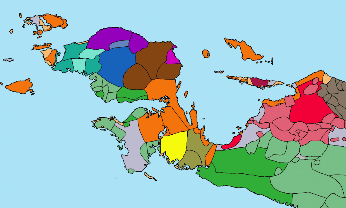
The right way to accomplish this would have been to fire up QGIS or other actual GIS software, and create a set of shapefiles corresponding to the geographic regions of interest. But since my “client”1 was under a time crunch, we settled on tracing over an existing map in Photoshop and filling in regions by hand with the Paint Bucket tool. Yes, this was a gross solution but it got the publication out on time, and the client is currently working on a proper GIS representation.2
In the meantime, the client wanted to generate a few alternative color schemes to highlight particular regions for another presentation (once again on a fairly rapid timetable) and I thought it would be a much easier task to accomplish in Illustrator rather than Photoshop, since vector graphics are much easier to work with when it comes to selecting colors for flat regions.
So I wrote a program to take the original map and convert it to a scalable vector graphics (SVG) file that can be easily imported into Illustrator. It ended up working out really nicely – here’s the final output (click to enlarge):

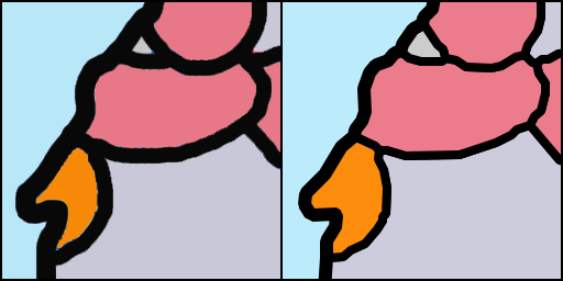
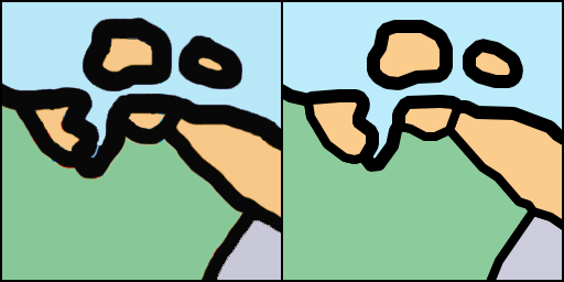
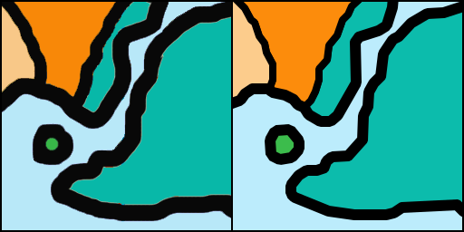
Let’s take a look at a few details from the two images. For each of these, the left-hand side comes from the original quick-and-dirty Photoshop output, and the right-hand side comes from rasterizing the SVG output of the program. You can see lots of tiny fringing artifacts from using the Paint Bucket tool to flood-fill regions in the original; they are completely gone in the vector output.
The SVG file affords a good deal of compression, too: the original PNG weighs in
at about 2.5M (reduced to 1.0M when lossily compressed by
pngquant). In contrast, the output SVG is
105K but just 38K when
gzip-compressed.
So not only does it look a lot nicer, the final output is about 25X
smaller than the original!
(Hmm, reminds me of my noteshrink project…)
Caveats
You should carefully consider whether maptrace is the right tool
for you!
First of all, it’s always better to use original georeferenced data if it’s available. Second, this is an incomplete system from a GIS standpoint because it doesn’t produce georeferenced output. If your input data is georeferenced, you will lose all of this information when the program is run.
Finally, please do not use this
software to circumvent copyright restrictions on existing maps! For
the purposes of copyright, you should consider the output of
maptrace a derivative work of the original input. So, only publish
maptrace output if you are licensed to reproduce the original input.
Producing watertight vector maps
There already exist tools to automatically convert raster (bitmap)
images to vector formats, including Adobe Illustrator’s
Live Trace/Image Trace
tools or standalone programs like Peter Selinger’s potrace, which provides the comparable functionality in Inkscape.
However, all of these tools share a common shortcoming from the perspective of mapmaking – given a simple raster line drawing like this heart:

…they actually produce two contours, one for the inside, and one for
the outside. You can demonstrate this by re-coloring the output of
potrace to stroke each contour:

What we would prefer is to replace the outline with a single contour that can be stroked
to any desired width. Here’s the output from my maptrace tool:

In actuality, maptrace also produces two contours surrounding the
heart (corresponding to the borders of the light and dark regions
above); however, they overlap completely, allowing the user to stroke
the border to whatever width they please.
Borrowing from the 3D modeling community, I’m going to refer to this property of completely overlapping outlines as a watertight map, since the boundary of each map region (i.e. the interior and exterior of the heart above) is completely coincident with its neighbor, leaving no gaps. Producing watertight maps was my main technical objective in undertaking this project.
Related efforts
As I was reading up when getting organized to write this post, I ran across a couple of related efforts:
-
https://cscott.net/Projects/Mallard/ – automatic generation of stained glass from photos, very similar goals and techniques
-
https://wiki.openstreetmap.org/wiki/User:TomChance/VectorisingStreetView – generating building outlines from raster data (no outlines, though)
-
https://wiki.openstreetmap.org/wiki/Mapseg – OpenStreetMap tool for segmenting maps, not sure how it deals with outlines
I’m sure this is an incomplete list, and there’s probably lots more interesting related work out there.
How it works
Here’s the step-by-step breakdown of how maptrace goes from a raster input to an output SVG.
1. Outline detection
First, the input image is thresholded to convert the original grayscale or RGB image into a 1-bpp boolean mask indicating where outlines are found. The resulting mask is nonzero wherever the maximum of the red, green, or blue channels exceeds a brightness threshold, OR wherever the alpha channel falls below some opacity threshold (e.g., we assume transparent areas are not map outlines).
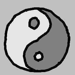
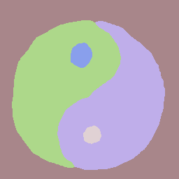
Let’s illustrate on this hastily drawn grayscale yin-yang symbol image:
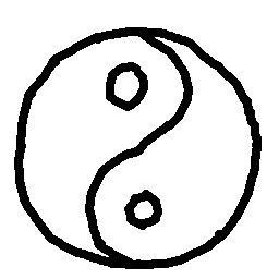
The mask produced by the thresholding operation is zero wherever the yin-yang outline falls, and one everywhere else:
Next, we can optionally apply
morphological operators
such as erosion, dilation, opening, or closing to the mask image. This
can be useful to dam small gaps in the outlines or join nearby
regions separated by very small bits of outline. We’re going to omit
this step for the yin-yang example, but see the
README.md in the github repository
for examples (look for the -f command-line option).
2. Connected component analysis
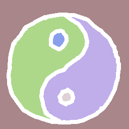
Now we take the mask computed above and perform connected-component labeling to identify the unique non-outline regions within the image. In our yin-yang example, there are five regions, each assigned a random color here (the outline itself is left white):
Our next step is to reduce the outline to a zero-thickness boundary.
3. Growing non-outline regions
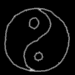
We now obtain the Euclidean Distance Transform (EDT) of the mask image. The EDT computes the distance from every outline pixel to the closest non-outline pixel. Here is a visualization (brighter pixels are embedded further inside the outline):
For our application of the EDT, we don’t care about the distances themselves; we are actually far more interested in the label of the closest non-outline pixel. When each outline pixel is assigned this label, the non-outline regions grow, and we obtain a map with no gaps between them at all:
Now it’s time to stop working with rasters and begin representing the image as a set of vector outlines.
4. Tracing borders between regions
Next, we trace along the outline of each labeled region (as well as the borders of the image) to create a set of nodes and edges. Each edge is a sequence of steps along the boundaries of pixels bordering two distinct regions, and the nodes are their intersection points (or arbitrary points along closed edges).
The SVG figure below shows the nodes as black circles and the edges as dotted lines whose colors indicate the labeled regions they border:

This tracing operation is by far the slowest part
of the program, since it’s all done with naïve loops in Python. It’s
theoretically possible to speed this operation up by parallelizing it or
calling out to Cython but I’d probably rather port
the entire program to a compiled langauge eventually instead.
5. Simplification
Next, we can optionally merge nearby nodes and then apply the Ramer-Douglas-Peucker algorithm to simplify each edge, with user-supplied tolerances. This is useful for eliminating the little square jaggies that result from following pixel-aligned paths. The results look like this:

6. SVG output
Finally, we generate the output SVG. For each labeled region, we loop over the edges that border it and concatenate them into one or more contours.3 We can assign random colors per region (as we have done so far in this example), pull colors in from the original image, or even assign them from another image of the same size and shape.
As a command-line option, we can tell the program to stroke the largest region (usually the background or ocean) with a larger outline, which often looks quite nice. Here’s the final output SVG for our yin-yang symbol example:

Here’s another example pulled from the github repository. The Original input image is the 2012 electoral map for Pennsylvania, pulled from Wikipedia:
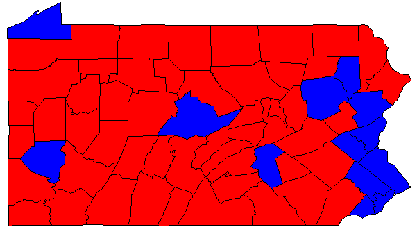
…and here’s the maptrace output as an SVG file:

Cool tricks & future work
After connected component labeling but before region growing, we can optionally delete very small regions whose areas fall below a certain threshold. This is nice for getting rid of single-pixel blips, but can also be used to remove text from maps, as in this US Census Bureau map of Pennsylvania counties, also taken from Wikipedia:
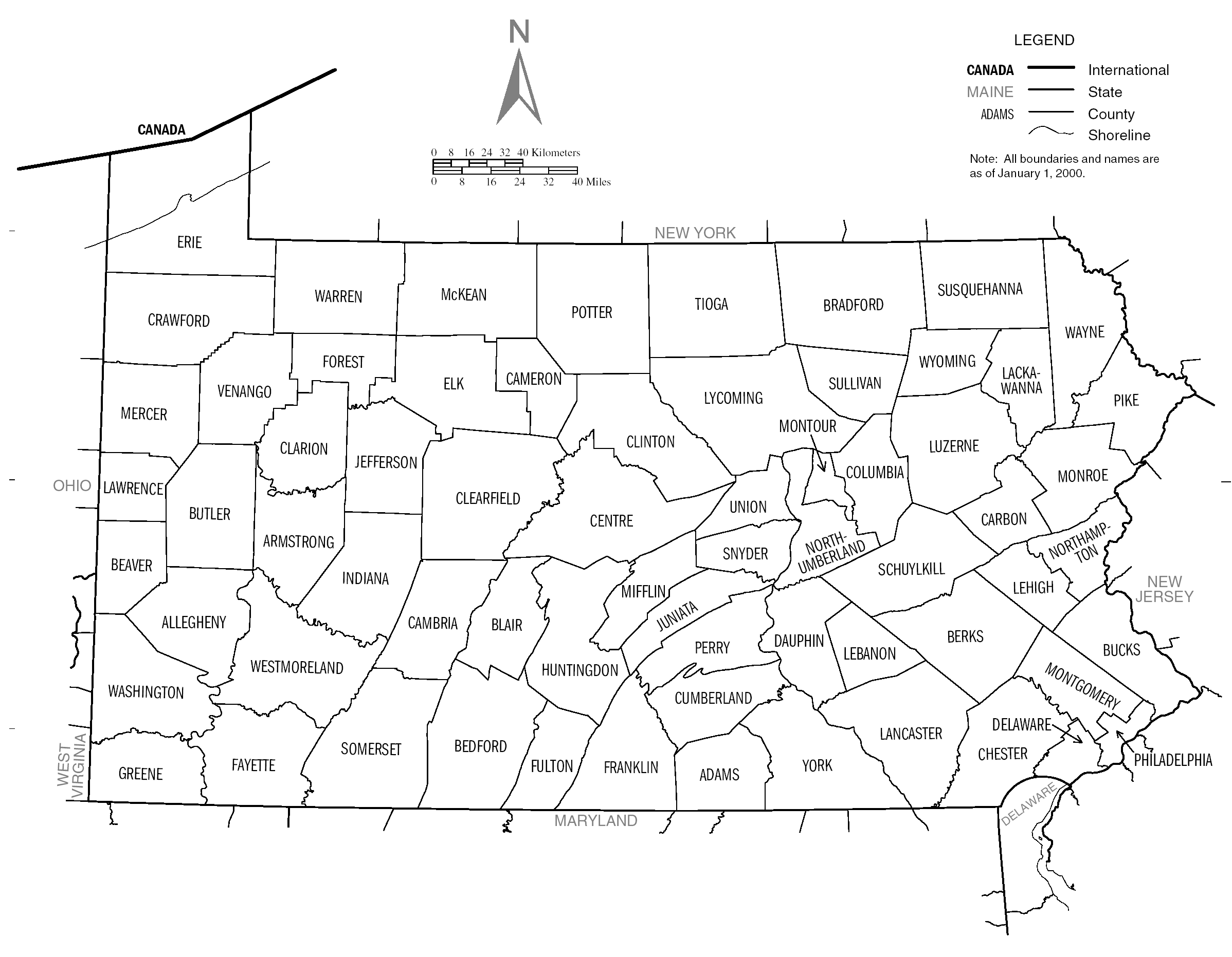
Here’s the resulting SVG file after deleting any enclosed region whose area is under 1000 pixels:

Magic, right?4
One area where potrace and its commercial analogues significantly
outperform maptrace is in their ability to recognize and output
curved paths. In contrast, every vector output by my program is
polygonal. They look fine when zoomed out, but don’t look great at low
resolution. Let’s call that future work.
Additionally, since it’s written in Python, maptrace is much slower
than an optimized implementation in a compiled language would be. Not
sure when I’ll get around to it, but I’ve been meaning to try out
Rust for a while, maybe I’ll take a crack at
porting it someday…
Anyways, that’s about it for now. Feel free to follow up on twitter with any questions or comments you might have!