Unprojecting text with ellipses

Using transformed ellipses to estimate perspective transformations of text.

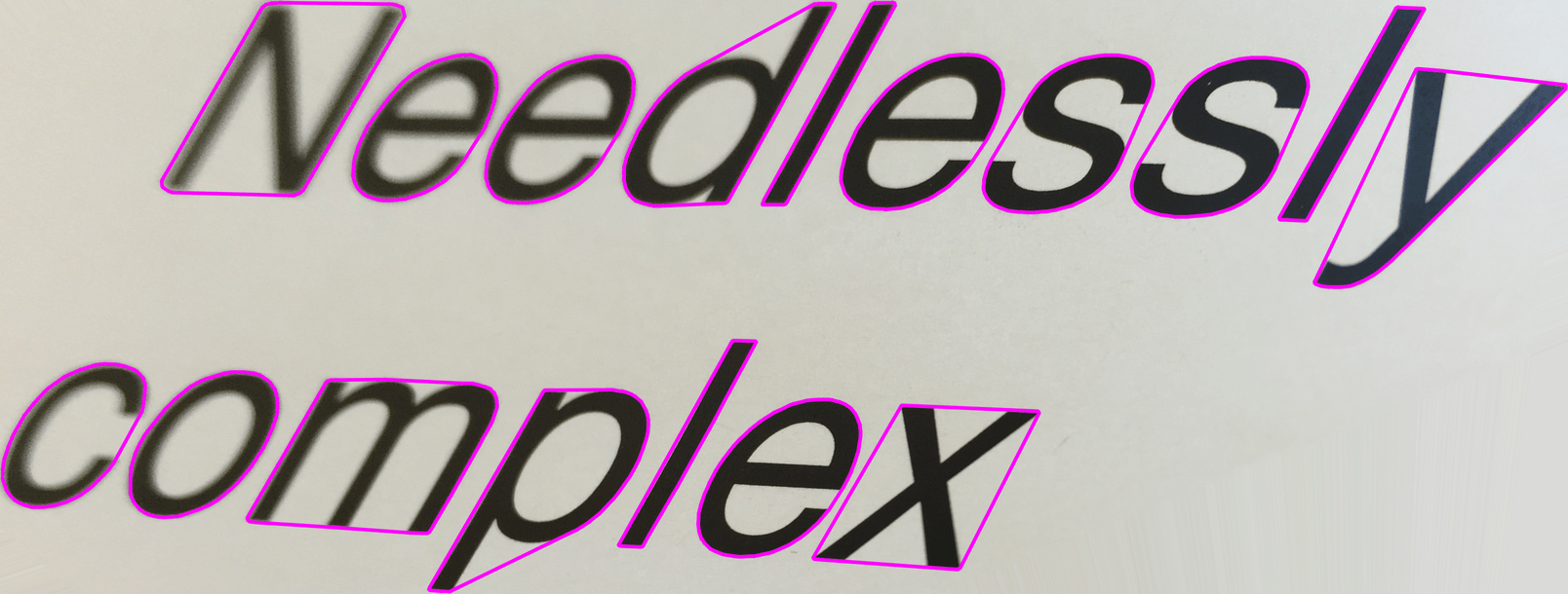
How do you automatically turn this:

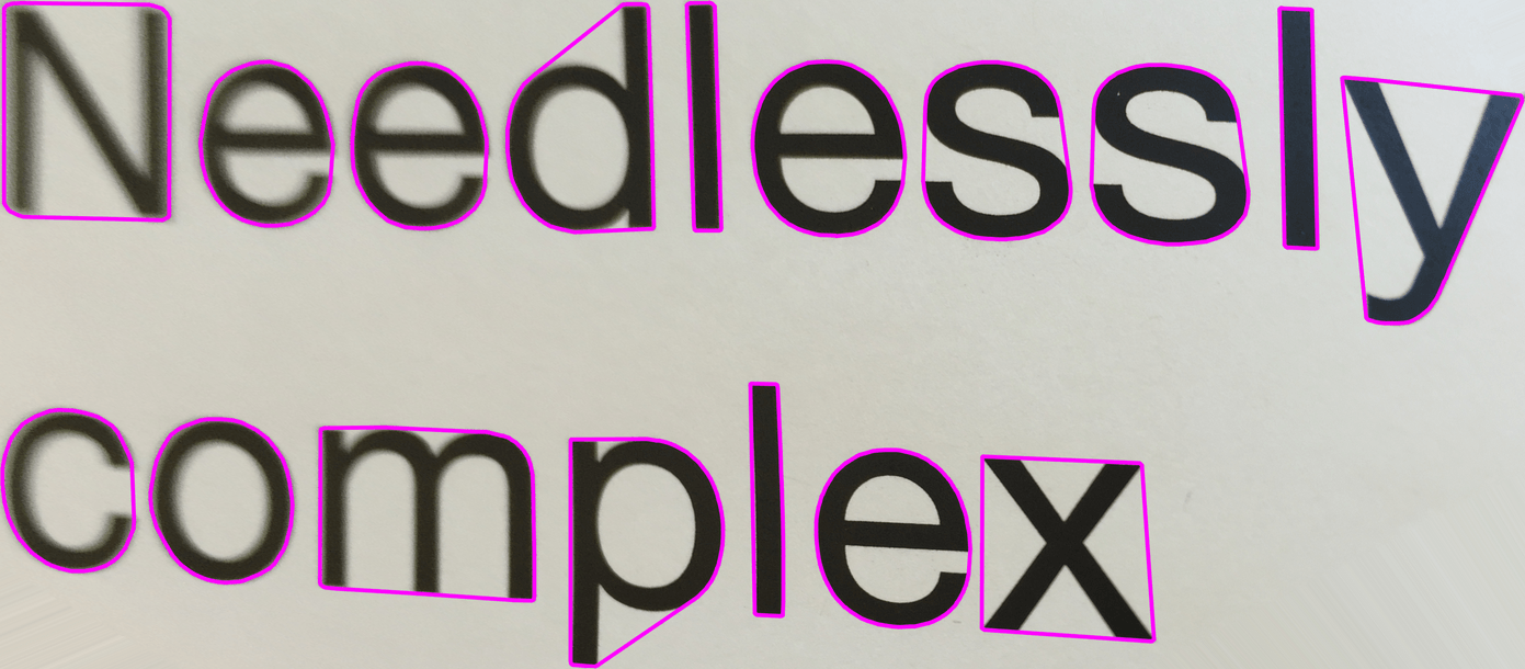
..into this?

Find out below, and be sure to check out the code on github afterwards…

Background

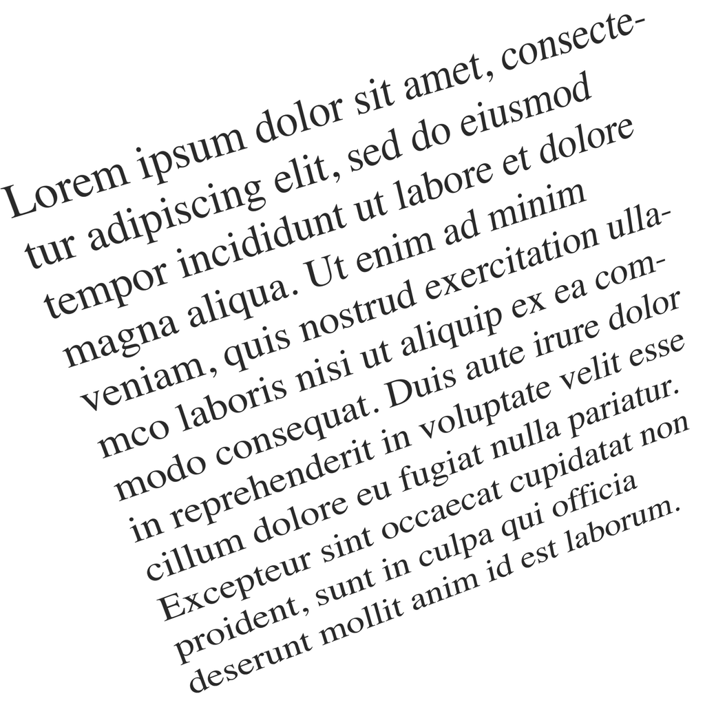
A while before my page dewarping project, I was already thinking about how to undo the effects of 3D projection on photographs of text. In the spring of 2016, I advised a couple of students working on a combined optical character recognition (OCR) and translation smartphone app for their Engineering senior design project. Their app was pretty cool – it used Tesseract OCR along with the Google Translate API to translate images in the user’s photo library. Users had to be careful, however, to photograph the text they wanted to translate head-on, so as to avoid strong perspective distortion of the type evidenced beautifully in the opening crawl for each of the Star Wars films:

Yep, just try running that thru OCR. Won’t work.

One my students found an interesting paper by Carlos Merino-Gracia et al. on how to undo this type of keystoning. When I looked it over, I wasn’t surprised that the students felt like they didn’t have time to implement it – to my eyes, the method seems sophisticated but also a bit complex.

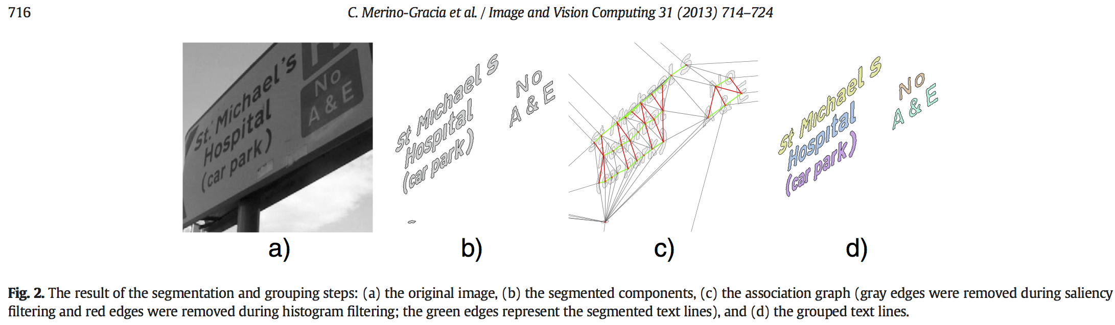
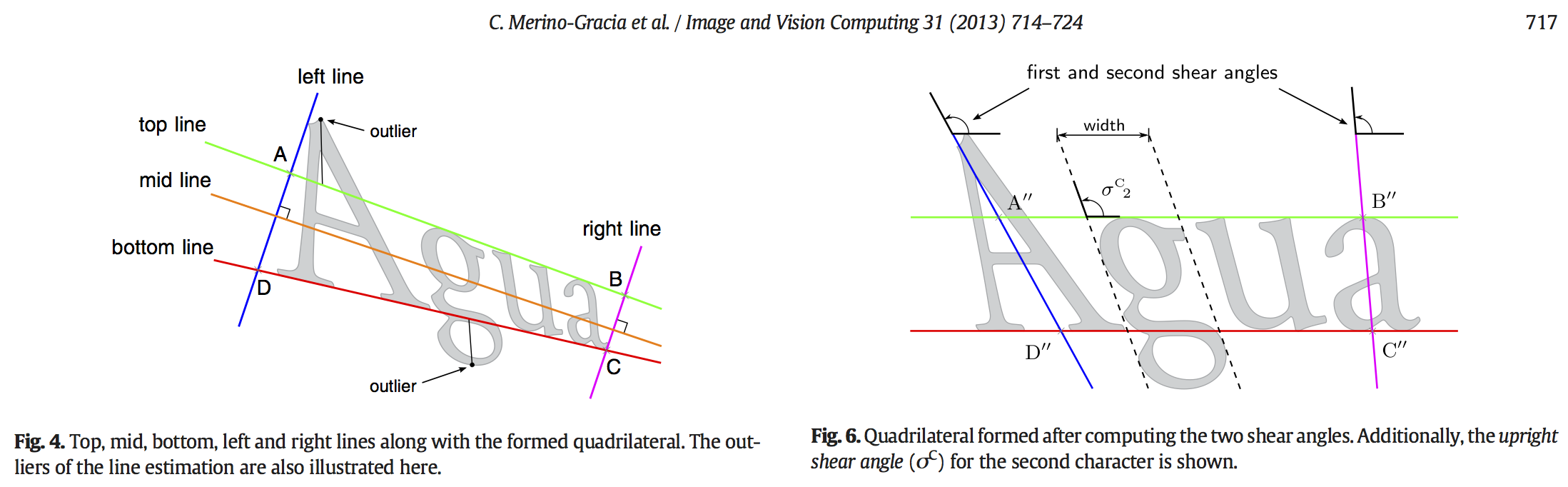
As these figures from the paper show, the method fits a quadrilateral to each line of the input text, which can then be rectified. This is useful but difficult because it requires detecting lines of text as the very first step. It’s kind of a “chicken and egg” problem: if the text were laid out horizontally, it would be trivial to detect lines; but the approach uses the detected lines in order to make the text horizontal!

My goal was to solve the perspective recovery problem based upon a much simpler model of text appearance, namely that on average, all letters should be about the same size. I was really happy with the approach I ended up with in this project, especially because I got to learn some interesting math along the way. Although I’m sure its neither as accurate or as useful as the Merino-Gracia approach, it ended up producing persuasive results on my test inputs in pretty rapid order.

Position/area correlations

Let’s restate the principle that’s going to guide our approach to the perspective removal problem:

On average, all letters should be about the same size.

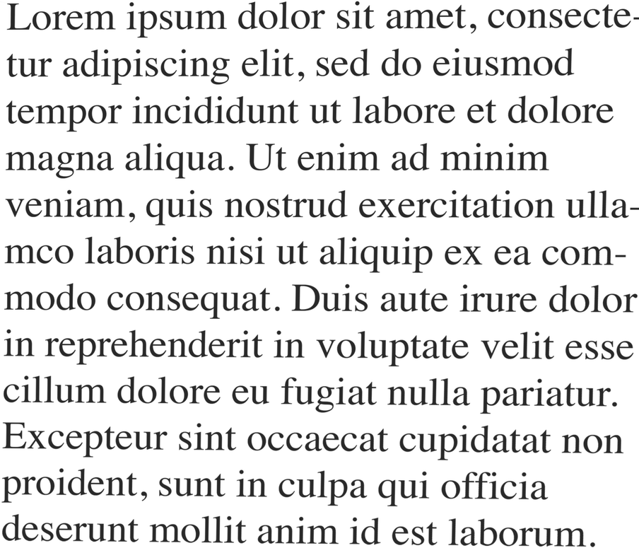
Because I don’t have a fancy text detector hanging around like Merino-Gracia et al.¹, I’m going to make a huge simplifying assumption that that the image we’re processing basically contains only the text that we want to rectify, like for example, this one:

In this case, we can use thresholding to obtain a clean bi-level image that separates letters from the background:

…and then use connected component labeling to obtain the outline – or contour, in image processing lingo – of each individual letter, like so:

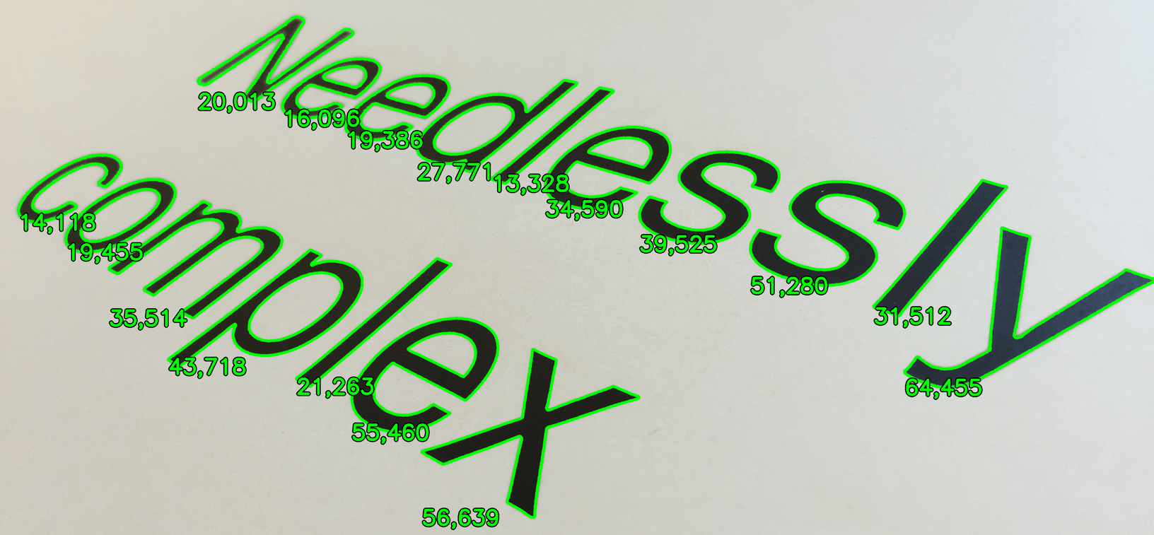
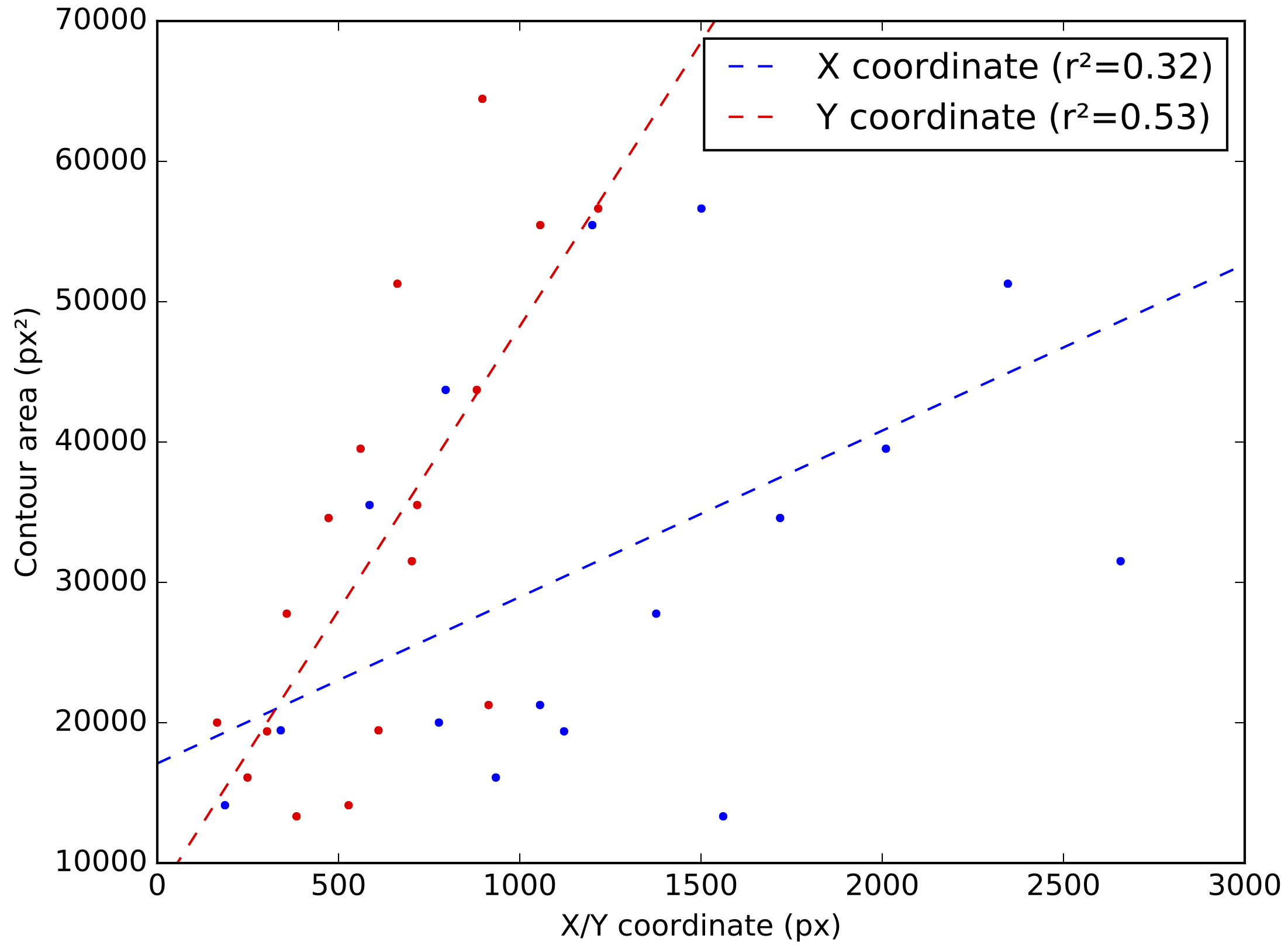
Here I’ve tagged each detected contour with its enclosed area, to make it clear that area correlates significantly with the position in the image. For example, the N and the c way over on the left cover drastically fewer pixels than the x and the y on the far right. If you plot the position-area relationship along with the best-fit regression lines, the correlation becomes even more apparent:

Our task is now pretty simple: if we want to remove the effects of perspective, all we have to do is to transform the image in such a way that the letter shapes tend to have uniform areas across the entire image – independent of their position.

But before we get started, we had better define what type of mathematical transformation we’re going to apply to our image to correct it.

Homographies: projections of planar objects

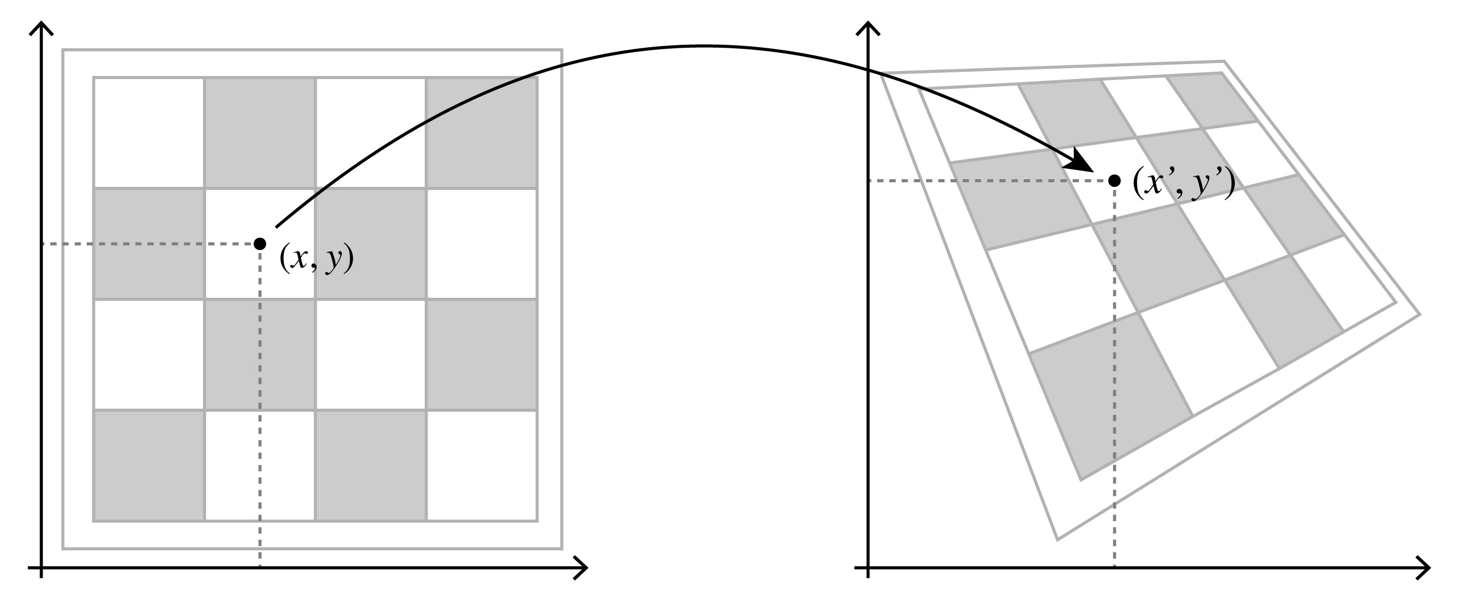
The mapping that turns normal-looking 2D text into the exciting Star Wars crawl that seems to zoom past the camera in 3D is called a homography. Due to the geometric optics underlying image formation, any time we take a photograph of a planar object like a chessboard or a street sign, it gets mapped through one of these. Mathematically, we can think about a homography transforming some original \((x, y)\) point on the surface of our planar object to a destination point \((x', y')\) inside of the image, like this:

There are a few different ways to represent homographies mathematically. Here’s a simple definition in terms of eight parameters \(a\) through \(h\):

\[x' = \frac{ax + by + c}{gx + hy + 1} , \quad y' = \frac{dx + ey + f}{gx + hy + 1}\]

As a superset of rotations, translations, scaling transformations, and shear transformations, homographies encompass a wide variety of effects. We can consider the influence of each parameter individually:

• \(a\) and \(e\) control scale along the \(x\) and \(y\) axes, respectively
• \(b\) and \(d\) control shear along each axis (together with \(a\) and \(e\) they also influence rotation, too)
• \(c\) and \(f\) control translation along each axis
• \(g\) and \(h\) control perspective distortion along each axis

The Shadertoy below shows how the appearance of Nyan Cat is altered as each parameter of the homography (from \(a\) to \(h\)) is changed individually. Press play in the bottom left corner to see the animation (you can also hit A to toggle extra animations because wheeee Nyan Cat).

By jointly changing all eight parameters, we can represent every possible perspective distortion of a planar object. Furthermore, since homographies are invertible, we can also use them to warp back from a distorted image to the original, undistorted planar object.

Homogeneous coordinates

Note: this section assumes a bit of linear algebra knowledge – you can skim it, but the math here will shore up the ensuing section about ellipses.

Remember how we said there are multiple ways to write down homographies? Well, here’s a matrix-based representation:

\[\tilde{\mathbf{p}}' = \left[\begin{array}{c} \tilde{x}' \\ \tilde{y}' \\ \tilde{w}' \end{array}\right] = \mathbf{H} \tilde{\mathbf{p}} = \left[\begin{array}{ccc} a & b & c \\ d & e & f \\ g & h & 1 \end{array}\right] \left[\begin{array}{c} x \\ y \\ 1 \end{array}\right] = \left[\begin{array}{c} ax + by + c \\ dx + ey + f \\ gx + hy + 1 \end{array}\right]\]

Denote by \(\mathbf{H}\) the \(3 \times 3\) matrix of parameters in the middle of the equation above. When we map the vector \(\tilde{\mathbf{p}} = (x, y, 1)\) through it, we get three outputs \(\tilde{x}'\), \(\tilde{y}'\), and \(\tilde{w}'\). In order to obtain our final coordinates \(x'\) and \(y'\), we simply divide the former two by \(\tilde{w}'\):

\[x' = \frac{\tilde{x}'}{\tilde{w}'} = \frac{ax + by + c}{gx + hy + 1}, \quad y' = \frac{\tilde{y}'}{\tilde{w}'} = \frac{dx + ey + f}{gx + hy + 1}\]

You can verify that this is exactly the same as our first definition of a homography above, just expressed a little bit more baroquely. Go ahead and make sure, I’ll wait…

Did it check out? Good.

Fine, the two definitions are the same – who cares? Well, it turns out we just wrote down the the homography using homogeneous coordinates, which establish a beautiful mathematical correspondence between matrices and a large family of non-linear transformations like homographies.

Anything you can do with the underlying transformations – such as composing two of them together – you can do in homogeneous coordinates with simple operations like matrix multiplication. And if the homogeneous representation of a transformation is an invertible matrix, then the parameters of the inverse transformation are straightforwardly obtained from the matrix inverse! So given our homography parameters \(a\) through \(h\), if we want to find the parameters of the inverse homography, all we need to do is compute \(\mathbf{H}^{-1}\) and grab its elements.²

Equalizing areas as an optimization problem

Let’s get back to our perspective recovery problem: we need to estimate a homography that will equalize the areas of all of the letters, once they’re all warped through it. Well, since \(g\) and \(h\) are the homography parameters that that determine the correlation between a shape’s position and its projected area, we should be able to find some setting for them that eliminates the correlation as much as possible. Therefore, we’ll fix the other six parameters for now, and just worry about producing the best possible perspective transformation of the form

\[\mathbf{H}_P = \left[\begin{array}{ccc} 1 & 0 & 0 \\ 0 & 1 & 0 \\ g & h & 1 \end{array}\right]\]

By “best”, we mean the matrix that minimizes the total sum of squares of the warped contours’ areas, defined as:

\[SS_{total} = \sum_{i=1}^n \left(A_i - \bar{A}\right)^2\]

where \(A_i\) is the area of the \(i^\text{th}\) warped contour (of which there are \(n\) total), and \(\bar{A}\) is the mean of all of their areas. Minimizing this total sum of squares is akin to minimizing the sample variance of the contour areas.

How do we accomplish this in practice? We just described an optimization problem: find the pair of parameters \((g, h)\) that minimizes the quantity above. There’s tons of ways to solve optimization problems, but when I’m in a hurry, I just hand them off to good old scipy.optimize.minimize. For all intents and purposes, we can consider it a “black box” that tries lots of different parameters, iteratively refining them until it finds the best combination.

Tracking areas through homographies

To evaluate our optimization objective, we’ll need to compute the areas of a bunch of contours. OpenCV accomplishes this via a variant of the shoelace formula, processing a contour consisting of \(m\) points in linear time of \(O(m)\). Despite this apparent efficiency, that’s actually bad news for us, because scipy.optimize.minimize has to compute the projected area for \(n\) contours (one for each letter) every time it wants to evaluate the optimization objective. If each contour consists of \(m\) points on average, our objective function would therefore take \(O(mn)\) time to run. To speed things up, we can replace each contour by a simpler “proxy” shape that is much easier to reason about. Here’s our letter contours once more:

We’ll be replacing them with these ellipses:

In the two images above, each red ellipse has the same area – that is, it covers the same number of pixels – as the green outlined letter that it replaces. There’s a few reasons I specifically chose ellipses as the proxy shape:

• They’re simple to describe – we can fully specify an ellipse with just five numbers.

• We can use them to not only match the area, but also the general aspect ratio and orientation of a letter (i.e. skinny or round, horizontal, vertical, or diagonal).

• Mapping an ellipse through a homography generally produces another ellipse.³

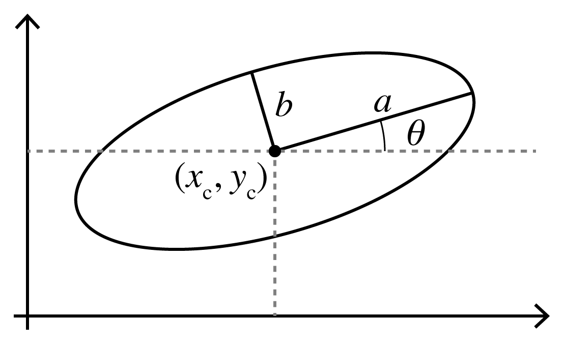
There are a couple of ways we can parameterize ellipses – let’s start with the canonical parameters \((x_c, y_c, a, b, \theta)\), where \((x_c, y_c)\) is the center point, \(a\) and \(b\) are the semi-major and semi-minor axis lengths, and \(\theta\) is the counterclockwise rotation of the ellipse from horizontal, as illustrated here:

Given a contour outlining a letter, we can find the “closest” matching ellipse by choosing these parameters such that the center point and areas match up. We can also examine the second-order shape moments of the contour to match the letter’s aspect ratio and orientation as well.

We can also represent an ellipse as the set of \((x, y)\) points that satisfy the implicit function

\[f(x, y) = Ax^2 + Bxy + Cy^2 + Dx + Ey + F = 0\]

where \(A\) through \(F\) are the parameters of our ellipse.⁴ We can switch back and forth between the two representations without changing the underlying mathematical object we’re describing – it’s just a matter of which one is more useful at the moment.

Just like we did with the homography, we can express the implicit function parameters as elements of a matrix that operates on homogeneous coordinates. The new function looks like this:

\[f(\tilde{\mathbf{p}}) = \tilde{\mathbf{p}}^T \mathbf{M} \tilde{\mathbf{p}} = \left[\begin{array}{ccc} x & y & 1 \end{array}\right] \left[ \begin{array}{ccc} A & B/2 & D/2 \\ B/2 & C & E/2 \\ D/2 & E/2 & F \end{array}\right] \left[\begin{array}{ccc} x \\ y \\ 1 \end{array}\right] = 0\]

As it turns out, if we want to map the entire ellipse through some homography \(\mathbf{H}\) represented as a \(3 \times 3\) matrix in homogeneous coordinates, we can compute the matrix

\[\mathbf{M}' = \mathbf{H}^{-T} \mathbf{M} \mathbf{H}^{-1}\]

and then straightforwardly obtain the parameters \(A'\) through \(F'\) of the the implicit function corresponding to the transformed ellipse by grabbing them out of the appropriate elements of \(\mathbf{M}'\).⁵

To illustrate how ellipses get mapped through homographies, I created another Shadertoy. When the faint rectangle and ellipse at the center of the display through a homography we see that the rectangle may transform into an arbitrary quadrilateral; however, the inscribed ellipse is just transformed into another ellipse. Interestingly, the center point of the new ellipse (red dot) is not the same as the transformed center point of the original ellipse (green dot). Once again, press the play button in the lower left to see the figure animate.

The bottom line of all this is that since there’s a closed-form formula for expressing the result of mapping an ellipse through a perspective transformation, it’s super efficient to model each letter as an ellipse for the purposes of running our objective function.

Here is what the optimization process looks like as it refines the warp parameters to improve the objective function:

The post-optimization, distortion-corrected image looks like this:

You can see we have equalized the letters’ areas quite a bit, just by considering the action of the homography \(\mathbf{H}_P\) on the collection of proxy ellipses.

Composing the final homography

Once the perspective distortion has been removed by finding the optimal \((g, h)\) parameters of the homography, we need to choose good values for the remaining parameters. In particular, we are concerned with the parameters \((a, b, d, e)\), which control rotation, scale, and skew. We will do this by composing the perspective transformation \(\mathbf{H}_P\) discovered in the previous step with two additional transformations: a rotation-only transformation \(\mathbf{H}_R\), and a skew transformation \(\mathbf{H}_S\). To find the optimal rotation angle, we will take a Hough transform of the contours after being mapped through \(\mathbf{H}_P\). Our input image is a binary mask indicating the edge pixels:

…and here is the corresponding Hough transform:

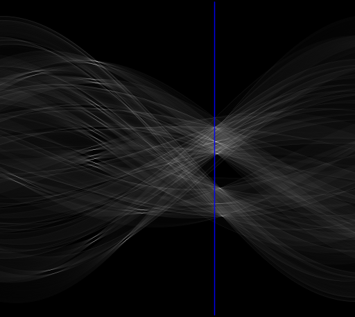
The Hough transform relates every possible line in the input image to a single pixel in the output image. Lines are parameterized by their orientation angle \(\theta\) (with 0° being horizontal and ±90° being vertical), as well as their distance \(r\) from the image origin. In the Hough transform output image, the brightness of a pixel at \((\theta, r)\) corresponds to the number of edge pixels detected along the line in the input image with angle \(\theta\) and distance \(r\) from the origin.

If a particular angle correlates well to the rotation of the text in the input image, its corresponding column in the Hough transform should be mostly zero pixels, with a small number of very bright pixels corresponding to the tops and bottoms of letters along parallel lines of the same angle. Conversely, angles which do not correlate well to the text rotation should have a more or less random spread of energy over all distances \(r\). To find the optimal rotation angle \(\theta\), we simply identify the column (highlighted above in blue) of the Hough transform containing the most zero pixels. We can then create a rotation matrix of the form

\[\mathbf{H}_R = \left[ \begin{array}{ccc} \phantom{-}\cos \theta & \sin \theta & 0 \\ -\sin \theta & \cos \theta & 0 \\ 0 & 0 & 1 \end{array}\right]\]

to rotate the image back by the detected \(\theta\) value. Here is the resulting image after warping first through \(\mathbf{H}_P\) and then \(\mathbf{H}_R\):

Finally, taking a cue from Merino-Gracia et al., we create a skew transformation

\[\mathbf{H}_S = \left[ \begin{array}{ccc} 1 & b & 0 \\ 0 & 1 & 0 \\ 0 & 0 & 1 \end{array}\right]\]

parameterized by a single skew parameter \(b\), that aims to reduce the width of the letters – this time using the convex hull of each detected contour as a proxy shape. Instead of minimizing the width of the widest letter, as Merino-Gracia et al. do, I found that on my inputs at least, using the soft maximum over hull widths gave nicer results than a straight-up maximum. Here’s the convex hulls after the rotation, but before the skew:

And the same convex hulls after discovering the optimal skew with scipy.optimize.minimize_scalar:

The final homography is given by composing the transformations we identified, applied in right-to-left order:⁶

\[\mathbf{H}_{final} = \mathbf{H}_S \, \mathbf{H}_R \, \mathbf{H}_P\]

Other examples

Here are a couple of other before/after image pairs. Input:

Output:

Input:

Output:

Conclusions and future work

What started out as an interesting alternative take and/or simplification of an existing paper’s approach turned into a fun deep dive into the math underlying homographies and ellipses. I especially enjoyed producing the visualizations and animations underlying my own approach. Again, I don’t want to claim that the work I did is state-of-the-art or even that it’s superior to existing methods like Merino-Gracia et al. – I just relish the process of wrapping my head around a technical challenge and carving it up into a sequence of well-defined optimization problems, as I’ve done in the past with my image fitting and page dewarping posts.

I hope you enjoyed scrolling through the blog post as much as I did creating it! Feel free to check out the code up on github.

1. See http://citeseerx.ist.psu.edu/viewdoc/summary?doi=10.1.1.102.3729 ↩

2. Small caveat: we first need to divide \(\mathbf{H}^{-1}\) by its bottom-right element so it becomes \(1\); or we just say “screw it” and represent homographies using nine parameters, ignoring scale. We were just gonna divide by \(\tilde{w}'\) anyways… ↩

3. Technically, mapping any conic section through a homography always gives another conic section. It’s possible that some homographies might turn a given ellipse “inside out” into a parabola or a hyperbola. ↩

4. Careful readers will have noticed that there are five canonical parameters but six implicit function parameters, and might be wondering whether we picked up an extra degree of freedom when we switched representations? The answer is no – since we can multiply the entire implicit function by an arbitrary non-zero constant without changing the zero set, there are six parameters, but only five underlying degrees of freedom. In this case, we say the implicit function parameters are “defined up to scale”. ↩

5. Here’s the proof: we want it to be true that for all \(\tilde{\mathbf{p}}' = \mathbf{H} \tilde{\mathbf{p}}\), the quantity \(\tilde{\mathbf{p}}'^T \mathbf{M}' \tilde{\mathbf{p}}' = \tilde{\mathbf{p}}^T \mathbf{M} \tilde{\mathbf{p}}\). That is, the value of the implicit function corresponding to the transformed ellipse, evaluated at the transformed point, should be the same as the original implicit function evaluated at the original point. This is true by construction if we define \(\mathbf{M}' = \mathbf{H}^{-T} \mathbf{M} \mathbf{H}^{-1}\) as above. ↩

6. You may have noticed we never discussed the translation parameters of the homography \(c\) and \(f\). That’s because I have to use them to “scroll” the entire image so it is visible below and to the right of the image origin at (0, 0). In fact, every image above that shows some warped image or contours is premultiplied by a translation transformation to make the image visible. ↩