Image fitting TensorFlow rewrite
Greater-than-100x speedup? Yes, please.
Introduction
A couple of weeks ago, in the course of writing my series of SymPy case studies, I mentioned that if I were going to write my image fitting C++ program today, I would just write it in Python using TensorFlow.
Well, I went ahead and did the rewrite this week, and as the post description above suggests, it was a great success. If you’re curious, you can skip straight to the github repository and try it out yourself before reading on, or go down to the results section to check out some videos of the training process.
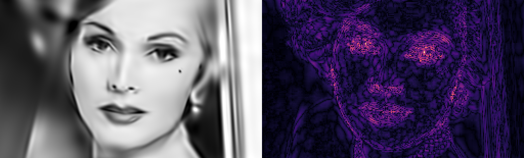
Left: final approximated image, Right: per-pixel error (brigher is higher).
Since I already described my approach to image fitting in detail, I’m not going to completely restate it here; instead, I’ll focus on major differences between this Python program and the original C++ program, as well as on some idiosyncratic TensorFlow usage conventions that you may not have seen elsewhere.
A bit of TensorFlow background
Note: if you’re familiar with TensorFlow’s programming model, you can skip to the next section.
Newcomers to TensorFlow and similar learning frameworks might find the underlying computation model a bit odd. For those readers, it’s worth taking a moment to learn about graph-based computing and how TensorFlow uses automatic differentiation for training.
TensorFlow introduces a novel datatype,
tf.Tensor,
to represent \(n\)-dimensional arrays. Say we want to compute
the sum of two tensors named a and b. This addition, like every
operation on tensors, gets separated into two steps: defining the
structure of the computation, and actually executing it.
# this defines a result tensor but computes nothing
c = tf.add(a, b)

# this actually does the computation
sess = tf.Session()
result = sess.run(c)
This indirection seems counterproductive, and is at the very least counterintuitive. Why the extra step?
Behind the scenes, TensorFlow is creating a dataflow graph to represent the operations that will be computed. You can think of this graph as an abstract recipe for how to produce each desired output from its inputs, almost like a makefile, but for tensor data instead of object files and executables.
The graph is abstract in the sense that it is agnostic as to whether the computation happens on the CPU, the GPU, or many CPUs/GPUs across a network – in fact, TensorFlow can target any of these, and the resulting speedup from parallelization often justifies the burden of wrapping your brain around the awkwardly indirect programming model.1
Aside from graph-based computation, the other big concept in
TensorFlow is using automatic differentiation to minimize loss
functions. The tf.Variable class is type of tensor that
is “train-able” by default: that is, TensorFlow can automatically
adjust its value to minimize any user-defined expression using
gradient descent and
its relatives.
Here’s a tiny TensorFlow program to fit a quadratic curve to the points \((-1, 2)\), \((0, 1)\), and \((2, 4)\):
from __future__ import print_function
import tensorflow as tf
import numpy as np

##################################################
# Step 1: define problem structure

# data to fit
xdata = np.array([-1, 0, 2], dtype=np.float32)
ydata = np.array([2, 1, 4], dtype=np.float32)

# define tf.Variable to hold polynomial coefficients
poly_coeffs = tf.get_variable(name='poly_coeffs', shape=(3))

# tf.Tensor expression for quadratic curve
y_poly = poly_coeffs[0]*xdata**2 + poly_coeffs[1]*xdata + poly_coeffs[2]

# tf.Tensor expression for squared error (we want this to go to zero)
err_sqr = tf.reduce_sum( (y_poly - ydata)**2 )

# define an operation to minimize the squared error
optimizer = tf.train.GradientDescentOptimizer(learning_rate=0.01)
train_op = optimizer.minimize(err_sqr)

##################################################
# Step 2: run computation

# create a TensorFlow session to host computaiton
sess = tf.Session()

# assigns random values to poly_coeffs
sess.run(tf.global_variables_initializer())

# optimize for a little while
for i in range(1000):
    e, _ = sess.run([err_sqr, train_op])
    print('error at iter {} is {}'.format(i+1, e))

# show final results
y, p = sess.run([y_poly, poly_coeffs])
print('fitted y values are:', y)
print('final poly coeffs are:', p)
Example output looks like this (your output will differ due to random variable initialization):
error at iter 1 is 8.30570030212
error at iter 2 is 4.77178478241
error at iter 3 is 3.39717292786
...
error at iter 1000 is 1.1425527191e-11
fitted y values are: [ 1.99999952  1.00000334  3.99999976]
final poly coeffs are: [ 0.83333147 -0.16666467  1.00000334]
Not perhaps the most fascinating example, especially given the
existence of np.polyfit, but it illustrates the two-stage
organization shared by all TensorFlow programs, and more importantly
it showcases TensorFlow’s ability to automatically find variable
values that minimize an arbitrary differentiable loss function.
Moving image fitting to TensorFlow
Now that we all understand a little bit about how TensorFlow works, let’s talk about rewriting the image fitting program to use it.
The old program, imfit.cpp, implements
hill climbing using a
nonlinear least squares
solver to change individual Gabor parameter vectors. It’s organized
along the lines of the following pseudocode:
until <Ctrl+C> pressed:

    choose a single set of parameters θ_i to fit from scratch or replace

    set cur_approx ← sum of Gabor functions for all params except θ_i
    set cur_target ← (input_image - cur_approx)

    set err_i ← || gabor(θ_i) - cur_target ||^2 if replacing; ∞ otherwise

    for each trial j from 1 to num_fits:

        randomly generate a new set of Gabor parameters θ_j
        solve nonlinear least squares problem to minimize
             err_j = || gabor(θ_j) - cur_target ||^2

        if err_j < err_i:
            set err_i ← err_j
            set θ_i ← θ_j
Although in principle the inner loop over randomly initialized parameter sets is embarassingly parallel, my original C++ program failed to exploit this property and just ran serially over each random initialization. In contrast, it’s trivial to parallelize this in TensorFlow, so we can essentially compute the appearance of every pixel for every random model \(j\) at the same time – a huge win.
Another big inefficiency of the program above is that it only ever solves a tiny nonlinear least squares problem – that is, it optimizes just eight parameters of a single Gabor function at a time. The main motivation for this was speed: on a single CPU with the levmar library, running a full, joint optimization of all 128 Gabor function parameter sets (\(8 \times 128 = 1024\) parameters with an error vector of \(128 \times 77 = 9856\) pixels) was agonizingly slow.2
In contrast, TensorFlow is pretty zippy when optimizing a full problem of this size both because it can parallelize computation on the GPU, and because the gradient descent algorithms that TensorFlow provides have much better asymptotic complexity than the algorithm used by levmar.
However, we can’t veer completely away from training/replacing individual parameter sets. This image approximation problem is prone to getting stuck in local minima – i.e., parameter sets for which any small change increases error, despite the availabily of better solutions elsewhere – as shown in this helpful Wikipedia diagram:

To mitigate this tendency to get stuck in local minima, the TensorFlow rewrite uses simulated annealing to replace individual Gabor parameter sets in between full joint parameter set updates. In practice, the program is willing to accept a small increase in overall error from time to time in order to “jump out” of local minima in the fitness landscape in hopes that the global optimizer will find an overall improved approximation as a result.
Here’s pseudocode for the new tf-imfit.py:
set update_count ← 0

until <Ctrl+C> pressed:

    choose a single set of parameters θ_i to fit from scratch or replace

    set cur_approx ← sum of Gabor functions for all params except θ_i
    set cur_target ← (input_image - cur_approx)

    set err_i ← || gabor(θ_i) - cur_target ||^2 if replacing; ∞ otherwise

    randomly fit num_fits individual Gabor parameters in parallel
    choose the one θ_j that has the lowest error err_j

    if err_j < err_i or we probabilistically accept a small increase:
       set θ_i ← θ_j

    if we have fit all 128 parameter sets so far:

       set update_count ← update_count + 1

       if update_count > updates_per_full_optimization:
         run a full optimization on the joint parameter set
         set update_count ← 0
One final difference between the programs worth mentioning is the way they handle constraints on the Gabor parameters. The levmar library can enforce linear inequality constraints (which is one main reason I selected it in the first place); however, TensorFlow can’t handle these natively. Instead, I choose to represent my linear inequalities as penalty functions that impose additional loss when violated. In practice, this means that there may be a tiny amount of constraint violation if it leads to lower error; however, since the constraints were only introduced for cosmetic reasons it’s no big deal.
A tour through the code
Let’s delve a little bit into the nitty-gritty details of how the new program is implemented, especially the TensorFlow-specific aspects.
First of all, let’s look at the image storage format. This
is handled by the GaborModel class defined around
line 227 of tf-imfit.py.
The self.gabor tensor that it computes is of shape \(n \times h \times w \times c\), where:
- \(n\) is the number of independent image fits being computed in parallel
- \(h \times w\) is the image shape (rows \(\times\) columns)
- \(c\) is the number of Gabor functions per fit
This is the so-called NHWC format in TensorFlow terminology.3
By summing across the final dimension, the GaborModel class produces a
self.approx tensor of shape \(n \times h \times w\), which we can
consider as \(n\) independent images which are each compared with the
current target in order to produce a sum of squared errors.
Together with the penalty functions from the inequality constraints,
these sums of squared errors combine to form the overall loss function
that is automatically minimized using the tf.train.AdamOptimizer
class (see
line 387).
Why represent the Gabor function output in this four-dimensional
format? In fact, it lets us solve two different optimization
sub-problems, depending on how we choose \(n\) and \(c\). If we set
\(n = 200\) and \(c = 1\), we can locally optimize many individual
Gabor parameter sets θ_j in parallel; when we set \(n = 1\) and \(c
= 128\) we are jointly optimizing the full collection of
parameters. As you can see starting around
line 540,
we accomplish this by instantiating two different GaborModel
objects, one to handle the parallel local fitting operation, and one
to handle the full joint optimization. The large-size preview images
used solely for visualization are generated by yet a third
GaborModel instance.
Next, let’s take a look at how we pass around paramater
data. Whenever it’s time to grab a Gabor parameter set from the
local parallel optimizer and hand it to the full joint optimizer, we
need to deal with the TensorFlow API because the parameters are
tf.Variable objects and not just simple Python variables which we
can easily modify.
Originally, I was using a
tf.assign
operation to pass the parameter values around inside my training loop,
but I noticed an odd behavior: although training started out very
quickly, it became slower and slower over time! A little googling
brought me to a couple of StackOverflow questions
[1,
2]
that indicated the flaw in my approach. By calling tf.assign inside
the training loop, I was adding to the dataflow graph during each
training iteration, inducing a quadratic runtime penalty (oops).
The fix for me was to use tf.Variable.load instead of tf.assign.
In hindsight, I could have figured out a way to keep using tf.assign to avoid a
round trip from GPU memory to CPU and back, but this was not a
significant bottleneck in my program. The StackOverflow questions
also pointed me to a good habit to prevent future slowdowns like this:
simply call tf.Graph.finalize() on the default graph before
training, as I now do on
line 862.
Finally, let’s discuss serialization and
visualization. In general, I think tf.train.Saver and TensorBoard are
flexible and powerful tools to accomplish these respective tasks, but
I find them to be overkill for small exploratory programs like this
one. The on-disk format used by tf.train.Saver is not well documented, and
takes up a ton of space because by default it serializes
not just your variables, but also the entire dataflow graph and
corresponding metadata. TensorBoard is also fairly heavyweight as it
builds upon the serialization functionality provided by tf.train.Saver.
Often, I find I want to store variables in a standard format that can
be easily saved or loaded in non-TensorFlow programs, and I also want a quick
way to produce debug visualizations.
In this program, I chose to store the parameters on disk in a
human-readable text file using np.savetxt (see
line 997).
To load them, I just call np.genfromtxt and then tf.Variable.load
to stash them into a TensorFlow variable (see
line 581).
I also decided on a simple way to produce debug visualizations using
numpy and Pillow’s Image. After each parameter update, I
generate a PNG image containing the current approximation as well as
the per-pixel error, which can be individually labeled in order to
provide a sense of updates over time. For details, see the snapshot
function defined around
line 409.
Results
As with the C++ version of the program, I found it most effective to
move from a coarse resolution to progressively higher resolutions,
similar to
the multigrid method
of solving differential equations. The
fitme.sh shell script
in the repository invokes tm-imfit.py several times to accomplish
this. All runtimes reported below were measured using TensorFlow 1.7
using a NVidia GTX 1080 GPU.
Running for 256 iterations at an image width of 64 pixels takes around 2 minutes and 14 seconds. Here’s a visualization of this initial fit:
What you’re seeing above is a succession of individual Gabor functions being incrementally fit one by one. After reaching the target total of 128 Gabor functions, the program begins performing global optimizations which rapidly decrease error. Thereafter, it alternates re-fitting 32 Gabor functions one-by-one with more joint optimizations. When re-fitting, the program uses simulated annealing to probabilistically allow minor increase in reconstruction error in order to escape local minima.
The odd ringing artifacts in the reconstructed image on the left-hand above are due to the fact that the Gabor functions are actually at a spatial frequency higher than the Nyquist rate for this small set of samples. Don’t worry about them too much, they’re about to disappear in the next level of optimization.
At this point, we run for 384 iterations at an image width of 96 pixels4. This round of optimization takes 7m18s. I decided not to show the individual Gabor function re-fits in this movie, but they are still happening behind the scenes:
Next, we run for 512 iterations at an image width of 128 pixels, for a duration of 14m31s:
Finally, we just run one single round of global optimization at an image width of 256 pixels, without any re-fits. This takes 1m54s:
All together, the total runtime for tf-imfit.py is 25 minutes and 57 seconds. In comparison, imfit.cpp achieved slightly lower quality after running for about three days (yes, days, not hours). Serendipitously,
my friend @a_cowley tweeted just this week:
Sometimes flipping the switch to run something on the GPU really does just make things 100x faster.
— Anthony Cowley (@a_cowley) April 26, 2018
Yep, that sounds about right.
By the way, the two programs are comparable in terms of source lines
of code. According to David A. Wheeler’s sloccount tool,
tf-imfit.py weighs in at 851 lines of Python, versus imfit.cpp
with 798 lines of C++. Although the Python program doesn’t have to
compute any derivatives, it does include more functionality because it
does both full and local optimizations.
That’s all for now – I had a good time putting together the program and this post. Hit me up on twitter if you have any questions or comments!
-
As of version 1.7, it looks like TensorFlow is promoting a brand-new Eager computation model to work around the separate graph-building step, but @BartWronsk reassures me the two stage model is unlikely to go away any time soon. ↩
-
The computational complexity of a single iteration of the Levenberg-Marquardt algorithm is something like \(O(m^3 + m^2k)\) where \(m\) is the number of parameters being fitted and \(k\) is the size of the error vector, so it scales pretty poorly to large problems. ↩
-
Originally, I had organized my data in the
NCHWformat, but after reading the performance guide, I realized it might be faster to re-order my data.NHWCgives me about a 3% speedup at larger image sizes on my GPU, so in the end it’s not a huge difference for this program. ↩ -
Yes I did pull these vaguely power-of-two-ish numbers out of thin air. ↩